REVIEW 3 major objections 6 minor 32 references
Taylor-Model Physics-Informed Neural Networks (PINNs) for Ordinary Differential Equations
T0 review · 3 major / 6 minor · reviewed 2026-08-06 · deepseek-v4-flash
Pith's one-line read A hybrid of symbolic Taylor series and a neural-network remainder yields ODE surrogate maps whose error starts at order t^(m+1) instead of order t.
desk verdict A clever, honest short-horizon surrogate method whose headline error bound is not actually proven—worth refereeing, but the theory needs to be downgraded or fixed. read the letter →
The pith
A machine-rendered reading of the paper's core claim, the machinery that carries it, and where it could break.
The reading
What carries the argument
The machinery is a Taylor-model expansion with a neural-network remainder. Symbolically computed Lie derivatives f_i (directional derivatives of the solution along the ODE flow) provide the polynomial part of the solution, and the network absorbs the rest. The losses are L_{r,g} = (1/N) Σ ‖ f(ϕ_r, θ, t) − (f_1 + t f_2 + ⋯ + t^m R_m / m! + $t^{{m+1}}$ Ẍ_m / (m+1)!) ‖ and L_{r,i} = (1/N) Σ ‖ f_{m+1}(x_0, θ, 0) − R_m(x_0, θ, 0) ‖. This converts matching the flow to order m+1 into a first-order regression problem for one network per state dimension, which is what carries the argument. A numerical-quadrature variant replaces Ẍ_m by trapezoidal integration of the integral representation of R_m, trading accuracy for training speed.
What would settle it
On a linear ODE with closed-form solution (for instance ẋ = x), train TM-PINNs at m = 1, 2, 3 with identical training budgets and measure max_{t∈[0,0.5]} |ϕ_r(t) − ψ(t)|. If the error does not fall roughly like $t^{{m+1}}$, the central error-growth claim is contradicted. A more direct check is to evaluate the derived ODE for R_m at t = 0: because τ_m = $t^{{m+1}}$ R_m / (m+1)!, the equation for Ẍ_m contains division by $t^{{m+1}}$ and is not Lipschitz at the origin, so the Grönwall bound used in the proof cannot be instantiated there.
Extended reading notes
Core claim
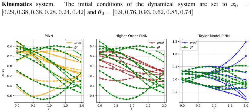
The central discovery is that the tail of a Taylor expansion is not an inert error term but a dynamical object: the m-th remainder τ_m of the solution satisfies ẏ_m(t) = f_1(ϕ_r, θ, t) − (f_1(0) + t f_2(0) + ⋯ + $t^{{m−1}}$/(m−1)! f_m(0)), with τ_m and its first m derivatives zero at t = 0. Writing τ_m = $t^{{m+1}}$ R_m / (m+1)!, the paper trains a network for R_m using two losses: a residual loss that compares ϕ̇_r with f(ϕ_r, θ, t), and an initial-condition loss that matches R_m(0) to f_{m+1}(x_0, θ, 0). The resulting “Taylor-Model PINN” represents the whole solution map ϕ_r as the symbolic polynomial plus the learned remainder. The authors claim this surrogate has error bounded by $t^{{m+1}}$(K_{r,i} + K_{r,g} t) $e^{{Kt}}$ / (m+1)!, and their experiments show it beating both plain PINNs and higher-order PINNs on MAE at one and two seconds on seven benchmark systems, using shallow one-hidden-layer networks. The tradeoff they report is slower training per epoch, offset by faster convergence.
Load-bearing premise
The entire error bound rests on applying the standard PINN Grönwall estimate to the ODE that the remainder network must solve, but that ODE divides by $t^{{m+1}}$ and is singular at t = 0, so the Lipschitz-right-hand-side premise of the estimate is not established for the remainder.
Editorial extensions
If this is right
- For control and parameter-estimation workflows that need many fast evaluations of a solution map, TM-PINNs offer a surrogate whose short-horizon error is orders of magnitude below vanilla PINNs, so gradient-based optimization over initial conditions and parameters becomes more reliable.
- Because the method uses only first-order derivatives of the network, adding Taylor order m raises the cost mainly in symbolic Lie-derivative computation, not in network Hessians.
- The error bound predicts the advantage is largest near t = 0 and decays as t increases; the reported MAE at three seconds, where TM-PINNs are no longer uniformly better, is consistent with that prediction.
- The architecture—one small network per state dimension—keeps evaluation cheap enough for real-time use, which is the motivation stated for replacing numerical solvers.
Reading between the lines
- Extending the same remainder decomposition to PDEs, which the authors leave as future work, would require assigning boundary conditions to the remainder; if that can be done, the t^{m+1} error-reduction mechanism should transfer to spatiotemporal problems.
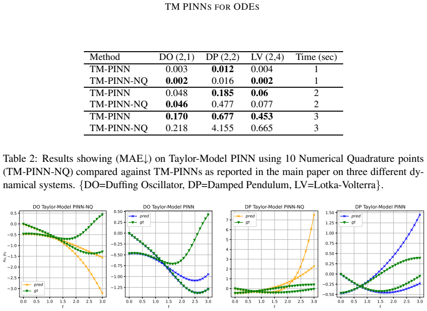
- The numerical-quadrature variant degrades sharply at t = 3 with only 10 quadrature points; a natural test is whether increasing K restores accuracy at acceptable cost, which would give a fully differentiation-free training scheme.
- The singularity at t = 0 in the remainder ODE suggests a practical diagnostic: if training on the residual loss alone fails near the origin even with the initial-condition loss satisfied, then the Grönwall premise is violated in practice, not just in the proof.
- The error-reduction mechanism is not tied to neural networks: any differentiable approximator of the remainder—a Gaussian process, a polynomial, a sparse grid—would inherit the t^{m+1} prefactor, so the method could combine with low-data regression in settings where training data are scarce.
Editorial analysis
A structured set of objections, weighed in public.
Referee Report
Summary. The paper proposes Taylor-Model PINNs (TM-PINNs) for learning surrogate solution maps of parametric ODEs. The method computes a symbolic Taylor polynomial of order m using Lie derivatives and represents the Taylor remainder R_m with a shallow neural network, trained through a residual loss L_{r,g} and an initial-condition loss L_{r,i}. The authors claim an error scaling of O(t^{m+1}e^{Kt}) for TM-PINNs versus O(te^{Kt}) for standard PINNs, and support this with experiments on seven ODE benchmarks plus two larger systems, reporting lower MAE for TM-PINNs at short prediction horizons. A numerical-quadrature variant is also discussed.
Significance. The core idea is attractive: combining symbolic Taylor expansion with a neural-network remainder avoids higher-order differentiation of the network and yields a surrogate that exactly matches the first m derivatives of the true solution by construction. If the error scaling were rigorously established, the method would be a useful practical tool for parametric ODE surrogates in control and parameter-estimation settings. The paper also provides code, considers a diverse set of benchmarks, and gives an alternative quadrature-based loss. However, the central theoretical claim is currently not proven, and the empirical evidence is weakened by the absence of error bars and by several results that contradict the stated 'up to two seconds' advantage.
major comments (3)
- [Section 3.1, Theorem 6] The proof of Theorem 6 is not valid as written. It says 'Applying Theorem 3 to the PINN learning problem for R_m', but Theorem 3 requires the network to satisfy an ODE whose right-hand side is Lipschitz continuous. Substituting τ_m = t^{m+1}R_m/(m+1)! into the ODE of Theorem 5 gives \dot R_m = ((m+1)!/t^{m+1}) [ f_1(φ_r,θ,t) - Σ_{j=1}^{m}(t^{j-1}/(j-1)!)f_j(0) - (t^m/m!)R_m ], whose right-hand side is singular at t=0: the coefficient of R_m behaves like (m+1)/t and the prefactor 1/t^{m+1} blows up. Thus the hypotheses of Theorem 3 are not satisfied for R_m. Applying Theorem 3 directly to φ_r yields only O(t e^{Kt}), because L_{r,i} controls R_m(0) rather than φ_r(0), and the t^{m+1} factor is lost. A correct proof must use the fact that φ_r matches the true solution's derivatives through order m (and through order m+1 when L_{r,i}=0) and must relate Krg,max to the weighted residual; no such argument is supplied. The central error-scaling claim is therefore not established.
- [Section 3.1, Example 3] The displayed Taylor expansion for the Duffing oscillator is internally inconsistent. In the second component, the coefficient of t is written as t(x−δy−x^3), using the current state (x,y) instead of the initial condition (x0,y0); the first component places f2(x0,δ,t) in the t^3 coefficient and omits the x-component of f3; and the notation f2/f3 does not distinguish the two state components. This makes the example unusable as a specification of the method, even though the general equations in Section 3.1 and Algorithm 1 are clearer. The example should be corrected to match Eq. (2).
- [Section 4.1, Table 1] The statement that TM-PINNs 'seem to match well ... up to two seconds for all the benchmark systems' is contradicted by Table 1: at t=2, TM-PINN MAE is larger than PINN MAE for Damped Pendulum (0.185 vs 0.143), Lorenz (0.074 vs 0.022), and SEIR (12.28 vs 0.135). Moreover, all numbers are point estimates with no error bars or repeated-seed statistics, so the reported ranking at t=1 and t=2 cannot be assessed for statistical reliability. The authors should report mean±std over multiple initializations and explicitly discuss the benchmarks where TM-PINN is not the best.
minor comments (6)
- [Section 2, Theorem 3 proof] The proof uses the symbol Ki,max, but only Li,max was defined; the same symbol should be used consistently throughout the proof.
- [Section 3.1, Eq. (2) and loss definitions] The notation f_i(0) versus f_i in Eq. (2) and in the definitions of L_{r,g} and L_{r,i} is inconsistent; all f_i appearing in the losses are understood to be evaluated at (x0,θ,0), and this should be stated explicitly.
- [Figures 9 and Table 1] The same model is called SEIR in Table 1 and SEIRS in Figure 9; the naming should be unified.
- [Appendix C.2] 'Negligent mean absolute error' should read 'negligible mean absolute error'.
- [Algorithm 1] The variable name 'gr' is reused for both the Taylor polynomial on line 6 and the right-hand-side evaluation on line 9, which is confusing; use distinct names.
- [Section 4, training-time discussion] The comparison of training times is hard to interpret because the number of epochs differs by orders of magnitude (500 TM-PINN epochs vs 10^5 PINN epochs); reporting total wall-clock time to reach a comparable validation error would be more informative.
Circularity Check
No significant circularity: TM-PINNs train only against physics residuals, and the claimed t^{m+1} error bound is an analytic proof claim with a proof gap, not a fit or a self-citation reduction.
full rationale
The derivation is self-contained. The remainder R_m is defined through the exact integral remainder formula in Eq. (1), and the training losses L_{r,g} and L_{r,i} measure the original ODE residual and the Taylor-coefficient initial condition; no ground-truth solution values are used as training targets, so the MAE comparisons against numerical solvers on the seven benchmarks are external and not fitted. The only self-citation by a co-author (Chen and Sankaranarayanan 2022) appears in the related-work discussion of Taylor-model reachability and is not load-bearing to the paper's main result. The proof of Theorem 6 does contain a genuine correctness gap: it says "Applying Theorem 3 to the PINN learning problem for R_m," but Theorem 3 requires the learned function to solve a first-order ODE with Lipschitz right-hand side, whereas the ODE implied for R_m by Theorem 5 becomes singular at t = 0 after dividing by t^{m+1}; moreover L_{r,g} bounds the tau_m residual, not the R_m residual. That is a rigor concern about the proof, not circularity, because the claimed bound is not obtained by substituting the target output into the loss. The paper also candidly reports that TM-PINNs degrade at longer horizons (Section 4.1), consistent with this proof gap. In short, no equation in the paper reduces to its own inputs, and no prediction is statistically forced by a fitted target.
Assumptions & free parameters
free parameters (4)
- Taylor expansion order m =
not specified; examples use m=4
- Loss weights =
1.0 for L_{r,g} and 1.0 for L_{r,i} (implied)
- Training budget =
TM-PINN about 500 epochs, PINN about 105 epochs, HO-PINN about 8 minutes
- Quadrature points K =
10 for the TM-PINN-NQ variant
assumptions (6)
- domain assumption The RHS f of the ODE is Lipschitz continuous, ensuring existence and uniqueness of solutions.
- domain assumption f is at least m+2 times continuously differentiable with respect to x, theta, and t.
- standard math Taylor's theorem with integral remainder (Apostol Theorem 7.6).
- standard math Gronwall's inequality.
- domain assumption The compact sets Omega, Theta, and [0,T] yield a compact range for x, so the ODE vector field is Lipschitz on the flow tube.
- ad hoc to paper A single-layer 64-neuron network can approximate the remainder R_m with small residual across the whole parametric family.
Cite this review
Pith. "Pith review of Taylor-Model Physics-Informed Neural Networks (PINNs) for Ordinary Differential Equations." pith.science (2026). https://pith.science/paper/ZA3NR2K6
@misc{pith2026250703860,
  author       = {Pith},
  title        = {Pith review of: Taylor-Model Physics-Informed Neural Networks (PINNs) for Ordinary Differential Equations},
  year         = {2026},
  howpublished = {\url{https://pith.science/paper/ZA3NR2K6}},
  note         = {Machine review of arXiv:2507.03860}
}
read the original abstract
We study the problem of learning neural network models for Ordinary Differential Equations (ODEs) with parametric uncertainties. Such neural network models capture the solution to the ODE over a given set of parameters, initial conditions, and range of times. Physics-Informed Neural Networks (PINNs) have emerged as a promising approach for learning such models that combine data-driven deep learning with symbolic physics models in a principled manner. However, the accuracy of PINNs degrade when they are used to solve an entire family of initial value problems characterized by varying parameters and initial conditions. In this paper, we combine symbolic differentiation and Taylor series methods to propose a class of higher-order models for capturing the solutions to ODEs. These models combine neural networks and symbolic terms: they use higher order Lie derivatives and a Taylor series expansion obtained symbolically, with the remainder term modeled as a neural network. The key insight is that the remainder term can itself be modeled as a solution to a first-order ODE. We show how the use of these higher order PINNs can improve accuracy using interesting, but challenging ODE benchmarks. We also show that the resulting model can be quite useful for situations such as controlling uncertain physical systems modeled as ODEs.
Figures


Figures from the paper (10 more)




Reference graph
Works this paper leans on
-
[1]
Ravi P. Agarwal and Donal O'Regan. Ordinary and Partial Differential Equations: With Special Functions, Fourier Series, and Boundary Value Problems. Universitext. Springer New York, NY, 1 edition, 2009
work page 2009
-
[2]
M. Althoff. An introduction to cora 2015. In Proc. of ARCH'15, volume 34 of EPiC Series in Computer Science, pages 120--151. EasyChair, 2015
work page 2015
-
[3]
Set propagation techniques for reachability analysis
Matthias Althoff, Goran Frehse, and Antoine Girard. Set propagation techniques for reachability analysis. Annual Review of Control, Robotics, and Autonomous Systems, 4, 2021
work page 2021
-
[4]
Eirini Angeloudi, Jeroen Audenaert, Micah Bowles, Benjamin M Boyd, David Chemaly, Brian Cherinka, Ioana Ciucă, Miles Cranmer, Aaron Do, Matthew Grayling, Erin E Hayes, Tom Hehir, Shirley Ho, Marc Huertas-Company, Kartheik G Iyer, Maja Jablonska, Francois Lanusse, Henry W Leung, Kaisey Mandel, Juan Rafael Martínez-Galarza, Peter Melchior, Lucas Meyer, Liam...
work page 2024
-
[5]
Tom M. Apostol. Calculus, Vol. 1: One-Variable Calculus, with an Introduction to Linear Algebra. John Wiley & Sons, New York, 2nd edition, 1991
work page 1991
-
[6]
Neural taylor approximations: Convergence and exploration in rectifier networks, 2016
David Balduzzi, Brian McWilliams, and Tony Butler-Yeoman. Neural taylor approximations: Convergence and exploration in rectifier networks, 2016
work page 2016
-
[7]
Analytic solutions to nonlinear odes via spectral power series
Estelle Basor and Rebecca Morrison. Analytic solutions to nonlinear odes via spectral power series. Linear Algebra and its Applications, 697: 0 561--582, Sep 2024
work page 2024
-
[8]
The stability of solutions of linear differential equations
Richard Bellman. The stability of solutions of linear differential equations. Duke Math. J., 10 0 (4): 0 643--647, 1943
work page 1943
Show all 32 references
-
[9]
Berz and K
M. Berz and K. Makino. Verified integration of ODE s and flows using differential algebraic methods on high-order T aylor models. Reliable Computing, 4: 0 361--369, 1998
1998
-
[10]
Reachability analysis for cyber-physical systems: Are we there yet? (invited paper)
Xin Chen and Sriram Sankaranarayanan. Reachability analysis for cyber-physical systems: Are we there yet? (invited paper). In Proc. NASA Formal Methods Symposium, volume 13260 of Lecture Notes in Computer Science, page 109–130. Springer, 2022
2022
-
[11]
Understanding the difficulty of training deep feedforward neural networks
Xavier Glorot and Yoshua Bengio. Understanding the difficulty of training deep feedforward neural networks. In Proceedings of the thirteenth international conference on artificial intelligence and statistics, pages 249--256. JMLR W&CP, 2010
2010
-
[12]
Hairer, G
E. Hairer, G. Wanner, and S. P. N rsett. Solving Ordinary Differential Equations I : Nonstiff Problems . Springer, Berlin, second edition, 1993
1993
-
[13]
Dual Cone Gradient Descent for Training Physics - Informed Neural Networks , jan 2025
Youngsik Hwang and Dong-Young Lim. Dual Cone Gradient Descent for Training Physics - Informed Neural Networks , jan 2025. arXiv:2409.18426 [cs]
2025 arXiv
-
[14]
Causally- Informed Deep Learning to Improve Climate Models and Projections
Fernando Iglesias-Suarez, Pierre Gentine, Breixo Solino-Fernandez, Tom Beucler, Michael Pritchard, Jakob Runge, and Veronika Eyring. Causally- Informed Deep Learning to Improve Climate Models and Projections . Journal of Geophysical Research: Atmospheres, 129 0 (4): 0 e2023JD0...
2024 doi
-
[15]
Kingma and Jimmy Ba
Diederik P. Kingma and Jimmy Ba. Adam: A method for stochastic optimization, 2014
2014
-
[16]
Systems Biology: A Textbook
Edda Klipp, Wolfram Liebermeister, Christoph Wierling, Axel Kowald, and Ralf Herwig. Systems Biology: A Textbook. Wiley-VCH, 2nd edition, 2016. ISBN 9783527336364. See Chapter 5: Modeling Biochemical Reactions — examples of cascades with Michaelis--Menten steps
2016
-
[17]
S. Kong, S. Gao, W. Chen, and E. M. Clarke. dreach: \( \) -reachability analysis for hybrid systems. In Proc. of TACAS'15, volume 9035 of LNCS, pages 200--205. Springer, 2015
2015
-
[18]
Characterizing possible failure modes in physics-informed neural networks
Aditi Krishnapriyan, Amir Gholami, Shandian Zhe, Robert Kirby, and Michael W Mahoney. Characterizing possible failure modes in physics-informed neural networks. In Advances in Neural Information Processing Systems , volume 34, pages 26548--26560. Curran Associates, Inc., 2021
2021
-
[19]
Medical image analysis using deep learning algorithms
Mengfang Li, Yuanyuan Jiang, Yanzhou Zhang, and Haisheng Zhu. Medical image analysis using deep learning algorithms. Front Public Health, 11: 0 1273253, nov 2023. ISSN 2296-2565. doi:10.3389/fpubh.2023.1273253
2023
-
[20]
Makino and M
K. Makino and M. Berz. Rigorous integration of flows and ODE s using T aylor models. In Proc.\ SNC'09, pages 79--84, 2009
2009
-
[21]
Raissi, P
M. Raissi, P. Perdikaris, and G. E. Karniadakis. Physics-informed neural networks: A deep learning framework for solving forward and inverse problems involving nonlinear partial differential equations. Journal of Computational Physics, 378: 0 686--707, feb 2019. ISSN 0021-9991...
2019 doi
-
[22]
Multistep neural networks for data-driven discovery of nonlinear dynamical systems, 2018
Maziar Raissi, Paris Perdikaris, and George Em Karniadakis. Multistep neural networks for data-driven discovery of nonlinear dynamical systems, 2018
2018
-
[23]
M. G. Rosenblum, A. Pikovsky, and J. Kurths. Synchronization -- A universal concept in nonlinear sciences. Cambridge University Press, Cambridge, 2001
2001
-
[24]
Physics- Informed Neural Network for Ultrasound Nondestructive Quantification of Surface Breaking Cracks
Khemraj Shukla, Patricio Clark Di Leoni, James Blackshire, Daniel Sparkman, and George Em Karniadakis. Physics- Informed Neural Network for Ultrasound Nondestructive Quantification of Surface Breaking Cracks . J Nondestruct Eval, 39 0 (3): 0 61, aug 2020. ISSN 1573-4862. doi:1...
2020 doi
-
[25]
Enhanced physics-informed neural networks with Augmented Lagrangian relaxation method ( AL - PINNs )
Hwijae Son, Sung Woong Cho, and Hyung Ju Hwang. Enhanced physics-informed neural networks with Augmented Lagrangian relaxation method ( AL - PINNs ). Neurocomputing, 548: 0 126424, sep 2023. ISSN 0925-2312. doi:10.1016/j.neucom.2023.126424
2023
-
[26]
Rohrhofer, and Bernhard C Geiger
Sophie Steger, Franz M. Rohrhofer, and Bernhard C Geiger. How PINN s cheat: Predicting chaotic motion of a double pendulum. In The Symbiosis of Deep Learning and Differential Equations II, 2022
2022
-
[27]
Is L2 Physics - Informed Loss Always Suitable for Training Physics - Informed Neural Network ? 2022
Chuwei Wang, Shanda Li, Di He, and Liwei Wang. Is L2 Physics - Informed Loss Always Suitable for Training Physics - Informed Neural Network ? 2022
2022
-
[28]
Deep learning of free boundary and Stefan problems
Sifan Wang and Paris Perdikaris. Deep learning of free boundary and Stefan problems. Journal of Computational Physics, 428: 0 109914, mar 2021. ISSN 00219991. doi:10.1016/j.jcp.2020.109914. arXiv:2006.05311 [math]
2021
-
[29]
Physics-informed Neural Implicit Flow neural network for parametric PDEs
Zixue Xiang, Wei Peng, Wen Yao, Xu Liu, and Xiaoya Zhang. Physics-informed Neural Implicit Flow neural network for parametric PDEs . Neural Netw, 185: 0 107166, jan 2025. ISSN 1879-2782. doi:10.1016/j.neunet.2025.107166
2025
-
[30]
Humphrey, and George Em Karniadakis
Minglang Yin, Xiaoning Zheng, Jay D. Humphrey, and George Em Karniadakis. Non-invasive Inference of Thrombus Material Properties with Physics -informed Neural Networks . Computer Methods in Applied Mechanics and Engineering, 375: 0 113603, mar 2021. ISSN 00457825. doi:10.1016/...
2021
-
[31]
Nn-poly: Approximating common neural networks with taylor polynomials to imbue dynamical system constraints
Frances Zhu, Dongheng Jing, Frederick Leve, and Silvia Ferrari. Nn-poly: Approximating common neural networks with taylor polynomials to imbue dynamical system constraints. Frontiers in Robotics and AI, 9, Nov 2022. doi:https://doi.org/10.3389/frobt.2022.968305
2022
-
[32]
Taylor expansion in neural networks: How higher orders yield better predictions
Pavel Zwerschke, Arvid Weyrauch, Markus Götz, and Charlotte Debus. Taylor expansion in neural networks: How higher orders yield better predictions. Iospress.nl, page 2983–2989, 2024. doi:https://doi.org/10.3233/FAIA240838
2024 doi
Reviewed August 6, 2026 · model on record in the stance chip above.
Discussion (0). Continue with ORCID to comment.