REVIEW 5 major objections 5 minor 64 references
Quantum Machine Learning for Identifying Transient Events in X-ray Light Curves
T0 review · 5 major / 5 minor · reviewed 2026-08-06 · deepseek-v4-flash
Pith's one-line read A quantum long short-term memory model trained on simulated AGN-like X-ray light curves finds 113 transient-event candidates in the XMM-Newton 4XMM-DR14 catalog, about 1.3 times the 85 found by a classical LSTM with the same…
desk verdict A transparent first application of QLSTM to X-ray transient detection, but the claimed quantum advantage over a classical LSTM is not statistically supported. read the letter →
The pith
A machine-rendered reading of the paper's core claim, the machinery that carries it, and where it could break.
The reading
What carries the argument
The central object is the quantum variational circuit (QVC), a small parameterized quantum circuit that replaces the fully connected layer inside each LSTM gate. Input data are encoded by a feature map; the best-performing map here, ZZFeatureMap, creates Hadamard superpositions, rotates qubits according to input values, and uses CNOT gates to entangle qubits, producing encodings that are hard to reproduce classically. A trainable ansatz then transforms the state; the C20 ansatz entangles neighboring qubits and rotates each qubit around three axes. Pauli-Z measurements on the qubits give the gate outputs, and the authors compare circuits with and without CNOT entanglements to isolate the effect of entanglement. They also measure expressive power with the effective dimension, which counts how many parameters actively shape the model's output for a given sample size.
What would settle it
Use the five known-QPE light curves that pass the paper's filtering (or a larger independently labeled set of real X-ray transients inside 4XMM-DR14) and count how many exceed the threshold-3.0 residual for the trained QLSTM versus the trained CLSTM; if the QLSTM does not recover more real events than the CLSTM at the same false-positive rate, the claimed quantum advantage is a simulation artifact rather than a detection fact.
Extended reading notes
Core claim
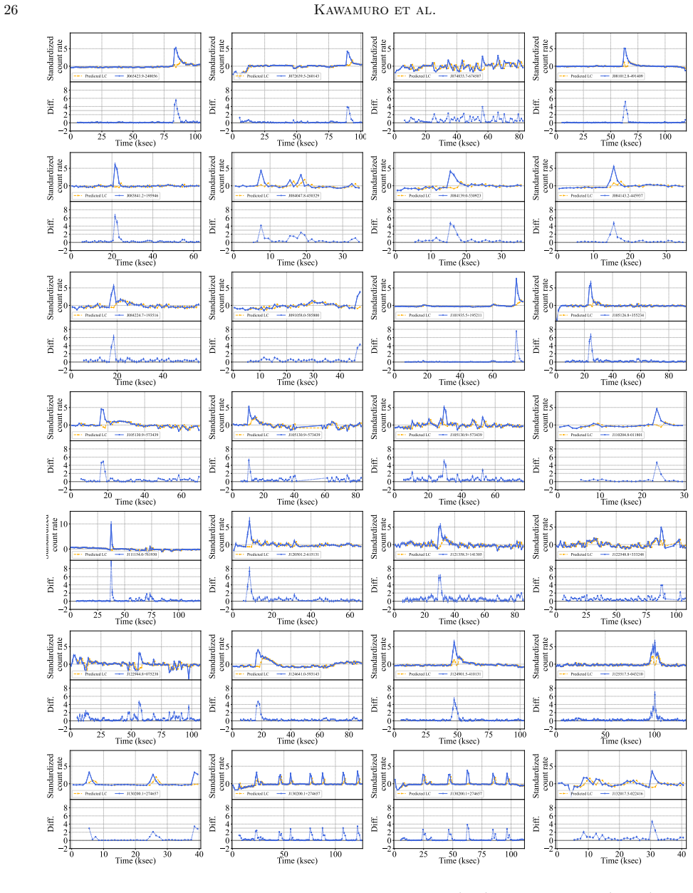
A quantum LSTM built by replacing the fully connected layers of each LSTM gate with quantum variational circuits can serve as an anomaly detector for X-ray time series. Trained only on simulated AGN-like variability and tested on single QPE-like flares, the QLSTM with the ZZFeatureMap and the C20 ansatz achieves a higher effective dimension, comparable false-positive rates, and consistently higher true-positive rates than a classical LSTM with the same parameter count; the advantage survives simulated device noise. When applied to 40,154 good-quality pn light curves from 4XMM-DR14 with a detection threshold of 3.0, this model identifies 113 light curves with anomalous flares, of which 101 have possible counterparts (mostly stellar activity) and 12 have no counterpart in SIMBAD or the ROSAT, SkyMapper, Pan-STARRS, and WISE surveys; one of the unmatched objects shows QPE-like flares. The authors also show the model recovers two of the five available light curves of the known QPE source RX J1301.9+2747.
Load-bearing premise
The comparison stands or falls on whether the computer-generated 'normal' AGN-like light curves and single QPE-like flares behave statistically like real X-ray sources; if real variability is different, the measured false-positive rate, the threshold of 3.0, and the 113-versus-85 gap could all change.
Editorial extensions
If this is right
- At threshold 3.0 the QLSTM reaches a true-positive rate near 0.8 for simulated flares of amplitude 1.5 while keeping the false-positive rate around 1e-3, so the same procedure should be usable as an automated transient filter on other X-ray catalogs.
- On 4XMM-DR14 the QLSTM yields 113 transient-event candidates versus 85 for the CLSTM, meaning the quantum model adds about 28 light curves worth examining at the same false-alarm level.
- The 12 candidates with no catalog counterpart, including the QPE-like object 4XMM J154910.4-534225, are the most promising targets for follow-up observation.
- Quantum noise from a current-device-derived noise model lowers prediction accuracy by only about 0.01 in loss, and the anomaly-detection ranking is largely preserved, so near-term noisy hardware does not by itself erase the quantum model's advantage.
- The recovery of two RX J1301.9+2747 light curves among the known QPE sample suggests that the model's sensitivity is adequate for at least the bright, fast class of quasi-periodic eruptions.
Reading between the lines
- At the paper's simulated false-positive rate of about 1e-3, a blind scan of roughly 40,000 light curves would be expected to produce around 40 false alarms, so the 113-candidate list is probably a mixture of real and spurious events rather than a clean catalog.
- The quantum-over-classical advantage is established on simulated single-flare anomalies; a direct test that injects flares into real light curves, or that runs both models on a labeled set of real transients, would show whether the 1.3-times yield survives outside simulation.
- The two recovered RX J1301.9+2747 observations suggest the same pipeline could be run on future XMM-Newton releases or on other soft-X-ray missions as a quasi-periodic-eruption candidate finder, an application the paper does not pursue.
- Because the QLSTM's extra detections are marginal at the chosen threshold, a slightly different threshold choice could erase or enlarge the quantum advantage; reporting the full threshold curve for the catalog run would make the comparison easier to interpret.
Editorial analysis
A structured set of objections, weighed in public.
Referee Report
Summary. The paper applies a quantum-variant long short-term memory (QLSTM) architecture, in which the fully connected layers of the LSTM gates are replaced by variational quantum circuits, to anomaly detection in X-ray light curves. Normal training data are simulated as AGN-like light curves and anomalous data as AGN-like curves with one injected QPE-like flare. Six QLSTM variants (differing in feature map and ansatz) and a classical LSTM (CLSTM) are trained on the same data. The authors report that QLSTM beats CLSTM in effective dimension, training loss, and true-positive rate, and they select a threshold of 3.0 from a simulated evaluation set (Set B). Applying the best QLSTM to 40,154 4XMM-DR14 pn light curves yields 113 anomaly candidates versus 85 for CLSTM; cross-matching leaves 12 candidates without counterparts. The central claim is that QLSTM 'slightly outperform[s]' CLSTM in expressive power, accuracy, and true-positive rate, and that the higher real-data detection count reflects this advantage.
Significance. If the QLSTM performance advantage were statistically established, this would be a novel and useful demonstration of quantum machine learning in time-domain X-ray astronomy, with a concrete product: a vetted catalog of 113 transient-event candidates and a comparison with a classical baseline. The paper is also commendable for discussing practical limitations of NISQ-based QLSTM (Section 8), documenting the quantum-circuit code (Appendix C), and providing a transparent description of the simulation and thresholding procedure. However, as presented, the central claim is not yet supported: the key comparison in Figure 9 has no uncertainty quantification, the abstract's 'accuracy' claim is contradicted by the validation-loss result, and the same simulated dataset is used for threshold selection and performance assessment. These issues are load-bearing for the paper's main conclusion and for the interpretation of the 113-versus-85 real-data counts.
major comments (5)
- [5.3 and Figure 9] The true-positive-rate advantage of QLSTM over CLSTM, which is the main quantitative support for the central claim, is shown only as point estimates with no confidence intervals or significance tests. Set B contains 1000 anomaly light curves per amplitude, so for rates near 0.8 the binomial standard error is about 1.3%; the QLSTM-CLSTM gap in Figure 9 appears to be of this order. Please add error bars (e.g., bootstrap or Wilson intervals), report the exact TPR/FPR values at the adopted threshold of 3.0 for each model, and include a significance test for the QLSTM-versus-CLSTM difference. Without this, the observed gap cannot be distinguished from sampling noise.
- [Abstract and Section 7] The abstract claims that QLSTM 'slightly outperform[s]' CLSTM in 'accuracy', but Section 7 explicitly states that for unseen validation data no significant differences are found, and the right panel of Figure 6 shows comparable validation losses. Training loss is not a valid proxy for predictive accuracy. The accuracy claim should be removed or reworded, or the authors should present a validation-based accuracy comparison that supports it. This matters because the abstract's triple claim (expressive power, accuracy, true-positive rate) is the paper's headline.
- [5.3 and 6] The threshold of 3.0 is selected using the same Set B that is then used to evaluate the false-positive and true-positive rates and to justify the QLSTM-versus-CLSTM comparison; the best model is also selected using Set A validation loss and Set B ROC-like curves. This creates a selection-bias loop: the reported TPR/FPR may be optimistically biased for the selected model and threshold. I recommend holding out an independent simulated test set (or a labeled real transient sample) for threshold selection, or at minimum reporting a cross-validated or nested evaluation.
- [Section 6] The 113-versus-85 counts from 4XMM-DR14 are interpreted as evidence for a QLSTM advantage, but real light curves are unlabeled, and the simulated anomaly training data (single QPE-like flares at fixed amplitudes, Section 3.1) may not represent the diversity of real X-ray transients. The only validation against real known QPEs uses five light curves surviving the filtering, of which two are detected; this is too small and too mixed to establish that the QLSTM finds more genuine transients rather than more false positives. The authors should either add a larger labeled real-transient validation set or explicitly state that the 113/85 comparison is an unvalidated model comparison, not a detection of more real transients.
- [3.2] The treatment of real light curves depends on the simulated training distribution (PSD slopes, excess variance range, and QPE flare model), and the final-5 ks exclusion is applied uniformly to all real light curves. If real X-ray variability differs from the simulated AGN-like model, or if genuine flares occur in the excluded final 5 ks, the reported detection counts and the QLSTM-CLSTM gap could change. Please quantify the sensitivity of the 113/85 result to the simulation assumptions, particularly the PSD slope prior and flare amplitude distribution, and justify the uniform 5-ks exclusion with an example or reference.
minor comments (5)
- [Figure 4 caption] The caption lists six QVCs as '(C20, C20), (AngleX, C20), (ZZFeatureMap, C20), (ZZFeatureMap, C20), (ZZFeatureMap, C20NoCNOT), and (AngleX, C20)', which duplicates ZZFeatureMap/C20 and omits (ZZFeatureMap, RealAmplitudes); the caption should match Table 1.
- [Section 7] The summary text contains the typo 'CLTM' instead of 'CLSTM' in the sentence 'This detection number is about 1.3 times higher than that by the CLTM model.'
- [Section 6] There is a typo in the sentence about an anomaly 'mioverlooked by the CLSTM model' that should read 'overlooked'.
- [3.2 / Figure 10] The text explains binning of real light curves but not how they are standardized before being fed to the model; since the model was trained on standardized simulated light curves, the standardization procedure for real data should be stated explicitly.
- [5.3] The false-positive rate at threshold 3.0 is quoted as approximately 1e-3, but with 1000 normal light curves in Set B the statistical precision of such a low rate is limited; reporting a confidence interval for the FPR would clarify how well this rate is actually constrained.
Circularity Check
No significant circularity: model, threshold, and catalog comparison are evaluated out-of-sample on independently drawn simulated data, with no fitted parameter renamed as a prediction.
full rationale
The derivation chain is not circular. The QLSTM and CLSTM models are trained on Set A simulated AGN-like light curves and evaluated on Set B (1000 normal and 1000 anomaly curves) and Set C, which are distinct draws from the same generative process rather than the training subset; no parameter is fitted to the real 4XMM-DR14 data before the models are applied. Defining anomalies as AGN-like variability plus one QPE-like flare is the target concept that supplies labels for a standard anomaly-detection benchmark, not a self-definitional reduction in which the output is equal to the input by construction. The threshold of 3.0 is selected from the Set B false-positive/true-positive curves and then applied identically to both QLSTM and CLSTM on real data, so the 113-vs-85 comparison is a relative benchmark under the same operating point; its absolute value inherits the simulation assumptions, but that is an extrapolation caveat, not circularity. Citations to Yen-Chi Chen et al. (2020) for the QLSTM architecture, Abbas et al. (2020) for effective dimension, and Timmer & König (1995) for light-curve simulation are external to the present author list and are not used as self-citations or uniqueness theorems. The only notable weakness is that the abstract's 'accuracy' component is qualified by the paper's own admission that validation losses show no significant differences, but that is an internal consistency and statistical-significance concern, not a circularity of the derivation.
Assumptions & free parameters
free parameters (3)
- Detection threshold =
3.0 (standardized residual)
- QPE flare amplitudes =
1.1, 1.5, 2.0, 3.0
- Model hyperparameters =
hidden size=2, qubits=4, ansatz reps=2 (6 for RealAmplitudes), 50 epochs, learning rate 0.05
assumptions (5)
- domain assumption AGN X-ray variability is a power-law PSD process with slopes drawn from Gaussian(mean=-2, std=0.3).
- domain assumption Excess variance is drawn uniformly in log space over [-5,-1].
- domain assumption QPE-like flares follow exponentially modified Gaussian profiles, one per light curve, with parameters from Webbe and Young (2023).
- domain assumption A prediction residual exceeding a fixed threshold is a valid indicator of an astrophysical transient, and the final 5 ks of every light curve can be excluded as non-celestial.
- domain assumption The effective dimension computed with a binary-classification simplification is a valid proxy for expressive power of the LSTM models.
Cite this review
Pith. "Pith review of Quantum Machine Learning for Identifying Transient Events in X-ray Light Curves." pith.science (2026). https://pith.science/paper/KYBSYSRM
@misc{pith2026250705589,
  author       = {Pith},
  title        = {Pith review of: Quantum Machine Learning for Identifying Transient Events in X-ray Light Curves},
  year         = {2026},
  howpublished = {\url{https://pith.science/paper/KYBSYSRM}},
  note         = {Machine review of arXiv:2507.05589}
}
abstract
We investigate whether a novel method of quantum machine learning (QML) can identify anomalous events in X-ray light curves as transient events and apply it to detect such events from the XMM-Newton 4XMM-DR14 catalog. The architecture we adopt is a quantum version of the long-short term memory (LSTM) where some fully connected layers are replaced with quantum circuits. The LSTM, making predictions based on preceding data, allows identification of anomalies by comparing predicted and actual time-series data. The necessary training data are generated by simulating active galactic nucleus-like light curves as the species would be a significant population in the XMM-Newton catalog. Additional anomaly data used to assess trained quantum LSTM (QLSTM) models are produced by adding flares like quasi-periodic eruptions to the training data. Comparing various aspects of the performances of the quantum and classical LSTM models, we find that QLSTM models incorporating quantum superposition and entanglement slightly outperform the classical LSTM (CLSTM) model in expressive power, accuracy, and true-positive rate. The highest-performance QLSTM model is then used to identify transient events in 4XMM-DR14. Out of 40154 light curves in the 0.2--12 keV band, we detect 113 light curves with anomalies, or transient event candidates. This number is $\approx$ 1.3 times that of anomalies detectable with the CLSTM model. By utilizing SIMBAD and four wide-field survey catalogs made by ROSAT, SkyMapper, Pan-STARRS, and WISE, no possible counterparts are found for 12 detected anomalies.
Figures


Figures from the paper (15 more)




Reference graph
Works this paper leans on
-
[1]
Abazajian, K., Adelman-McCarthy, J. K., Ag¨ ueros, M. A., et al. 2003, AJ, 126, 2081, doi: 10.1086/378165
doi:10.1086/378165 2003
-
[2]
2020, arXiv e-prints, arXiv:2011.00027, doi: 10.48550/arXiv.2011.00027
Abbas, A., Sutter, D., Zoufal, C., et al. 2020, arXiv e-prints, arXiv:2011.00027, doi: 10.48550/arXiv.2011.00027
-
[3]
2020, ApJ, 896, 39, doi: 10.3847/1538-4357/ab91ba
Alp, D., & Larsson, J. 2020, ApJ, 896, 39, doi: 10.3847/1538-4357/ab91ba
-
[4]
Aniyan, A. K., & Thorat, K. 2017, ApJS, 230, 20, doi: 10.3847/1538-4365/aa7333
-
[5]
2021, Nature, 592, 704, doi: 10.1038/s41586-021-03394-6 Astropy Collaboration, Robitaille, T
Arcodia, R., Merloni, A., Nandra, K., et al. 2021, Nature, 592, 704, doi: 10.1038/s41586-021-03394-6 Astropy Collaboration, Robitaille, T. P., Tollerud, E. J., et al. 2013, A&A, 558, A33, doi: 10.1051/0004-6361/201322068 Astropy Collaboration, Price-Whelan, A. M., Sip˝ ocz, B. M., et al. 2018, AJ, 156, 123, doi: 10.3847/1538-3881/aabc4f
-
[6]
2022, MNRAS, 509, 3504, doi: 10.1093/mnras/stab3259
Bao, T., & Li, Z. 2022, MNRAS, 509, 3504, doi: 10.1093/mnras/stab3259
-
[7]
Becker, R. H., White, R. L., & Helfand, D. J. 1995, ApJ, 450, 559, doi: 10.1086/176166
doi:10.1086/176166 1995
-
[8]
2020, arXiv e-prints, arXiv:2001.10872, doi: 10.48550/arXiv.2001.10872
Berezniuk, O., Figalli, A., Ghigliazza, R., & Musaelian, K. 2020, arXiv e-prints, arXiv:2001.10872, doi: 10.48550/arXiv.2001.10872
Show all 64 references
-
[9]
2014, Advances in Space Research, 53, 900, doi: 10.1016/j.asr.2013.07.045
Bianchi, L., Conti, A., & Shiao, B. 2014, Advances in Space Research, 53, 900, doi: 10.1016/j.asr.2013.07.045
2014 doi
-
[10]
J., Geim, A
Bluvstein, D., Evered, S. J., Geim, A. A., et al. 2024, Nature, 626, 58, doi: 10.1038/s41586-023-06927-3
2024 doi
-
[11]
J., Tr¨ umper, J., et al
Boller, T., Freyberg, M. J., Tr¨ umper, J., et al. 2016, A&A, 588, A103, doi: 10.1051/0004-6361/201525648
2016 doi
- [12]
-
[13]
Davenport, J. R. A. 2016, ApJ, 829, 23, doi: 10.3847/0004-637X/829/1/23
2016 doi
-
[14]
R., Chornock, R., Soderberg, A
Drout, M. R., Chornock, R., Soderberg, A. M., et al. 2014, ApJ, 794, 23, doi: 10.1088/0004-637X/794/1/23
2014 doi
-
[15]
A., Mahabal, A., Masci, F
Duev, D. A., Mahabal, A., Masci, F. J., et al. 2019, MNRAS, 489, 3582, doi: 10.1093/mnras/stz2357
2019 doi
-
[16]
P., et al
Fender, R., Stewart, A., Macquart, J. P., et al. 2015, in Advancing Astrophysics with the Square Kilometre Array (AASKA14), 51, doi: 10.22323/1.215.0051
2015 doi
-
[17]
A., Magnier, E
Flewelling, H. A., Magnier, E. A., Chambers, K. C., et al. 2020, ApJS, 251, 7, doi: 10.3847/1538-4365/abb82d Gonz´ alez-Mart ´ ın, O., & Vaughan, S. 2012, A&A, 544, A80, doi: 10.1051/0004-6361/201219008
2020 doi
- [18]
-
[19]
2023, ApJ, 942, 9, doi: 10.3847/1538-4357/aca283
Hammerstein, E., van Velzen, S., Gezari, S., et al. 2023, ApJ, 942, 9, doi: 10.3847/1538-4357/aca283
2023 doi
-
[20]
R., Millman, K
Harris, C. R., Millman, K. J., van der Walt, S. J., et al. 2020, Nature, 585, 357, doi: 10.1038/s41586-020-2649-2 Havl ´ ıˇ cek, V., C´ orcoles, A. D., Temme, K., et al. 2019, Nature, 567, 209, doi: 10.1038/s41586-019-0980-2
2020 doi
-
[21]
Ho, A. Y. Q., Perley, D. A., Gal-Yam, A., et al. 2023, ApJ, 949, 120, doi: 10.3847/1538-4357/acc533
2023 doi
-
[22]
1997, Neural computation, 9, 1735
Hochreiter, S., & Schmidhuber, J. 1997, Neural computation, 9, 1735
1997
-
[23]
2021, Nature Communications, 12, 2631, doi: 10.1038/s41467-021-22539-9
Huang, H.-Y., Broughton, M., Mohseni, M., et al. 2021, Nature Communications, 12, 2631, doi: 10.1038/s41467-021-22539-9
2021 doi
- [24]
-
[25]
2001, A&A, 365, L1, doi: 10.1051/0004-6361:20000036
Jansen, F., Lumb, D., Altieri, B., et al. 2001, A&A, 365, L1, doi: 10.1051/0004-6361:20000036
2001 doi
-
[26]
2016, PASJ, 68, 58, doi: 10.1093/pasj/psw056 —
Kawamuro, T., Ueda, Y., Shidatsu, M., et al. 2016, PASJ, 68, 58, doi: 10.1093/pasj/psw056 —. 2018, ApJS, 238, 32, doi: 10.3847/1538-4365/aad1ef
2016 doi
-
[27]
2023, Nature, 618, 500, doi: 10.1038/s41586-023-06096-3 Kovaˇ cevi´ c, M., Pasquato, M., Marelli, M., et al
Kim, Y., Eddins, A., Anand, S., et al. 2023, Nature, 618, 500, doi: 10.1038/s41586-023-06096-3 Kovaˇ cevi´ c, M., Pasquato, M., Marelli, M., et al. 2022, A&A, 659, A66, doi: 10.1051/0004-6361/202142444
2023 doi
- [28]
- [29]
-
[30]
D., et al
Lien, A., Sakamoto, T., Barthelmy, S. D., et al. 2016, ApJ, 829, 7, doi: 10.3847/0004-637X/829/1/7
2016 doi
-
[31]
A., & Barret, D
Lin, D., Webb, N. A., & Barret, D. 2012, ApJ, 756, 27, doi: 10.1088/0004-637X/756/1/27
2012 doi
-
[32]
2019, ApJ, 870, 126, doi: 10.3847/1538-4357/aaf39b
Lin, J., Yan, Z., Han, Z., & Yu, W. 2019, ApJ, 870, 126, doi: 10.3847/1538-4357/aaf39b
2019 doi
-
[33]
2020, JCAP, 2020, 050, doi: 10.1088/1475-7516/2020/03/050
Maggiore, M., Van Den Broeck, C., Bartolo, N., et al. 2020, JCAP, 2020, 050, doi: 10.1088/1475-7516/2020/03/050
2020 doi
-
[34]
2011, ApJ, 731, 53, doi: 10.1088/0004-637X/731/1/53
Mainzer, A., Bauer, J., Grav, T., et al. 2011, ApJ, 731, 53, doi: 10.1088/0004-637X/731/1/53
2011 doi
-
[35]
2022, A&A, 664, A81, doi: 10.1051/0004-6361/202142952
Makhlouf, K., Turpin, D., Corre, D., et al. 2022, A&A, 664, A81, doi: 10.1051/0004-6361/202142952
2022 doi
-
[36]
Metzger, B. D. 2017, Living Reviews in Relativity, 20, 3, doi: 10.1007/s41114-017-0006-z
2017 doi
-
[37]
Moshir, M., Kopman, G., & Conrow, T. A. O. 1992, IRAS Faint Source Survey, Explanatory supplement version 2 Quantum machine learning for anomaly detection 35
1992
-
[38]
S., Lochner, M., Webb, S., & Narayan, G
Muthukrishna, D., Mandel, K. S., Lochner, M., Webb, S., & Narayan, G. 2022, MNRAS, 517, 393, doi: 10.1093/mnras/stac2582
2022 doi
- [39]
-
[40]
2014, ApJ, 793, 23, doi: 10.1088/0004-637X/793/1/23
Nun, I., Pichara, K., Protopapas, P., & Kim, D.-W. 2014, ApJ, 793, 23, doi: 10.1088/0004-637X/793/1/23
2014 doi
-
[41]
2024, ApJS, 272, 13, doi: 10.3847/1538-4365/ad344f
Panda, S., & ´Sniegowska, M. 2024, ApJS, 272, 13, doi: 10.3847/1538-4365/ad344f
2024 doi
-
[42]
L., Lieu, M., & Matzeu, G
Parker, M. L., Lieu, M., & Matzeu, G. A. 2022, MNRAS, 514, 4061, doi: 10.1093/mnras/stac1639
2022 doi
-
[43]
2019, arXiv e-prints, arXiv:1912.01703, doi: 10.48550/arXiv.1912.01703 Peral Garc ´ ıa, D., Cruz-Benito, J., & Jos´ e Garc ´ ıa-Pe˜ nalvo, F
Paszke, A., Gross, S., Massa, F., et al. 2019, arXiv e-prints, arXiv:1912.01703, doi: 10.48550/arXiv.1912.01703 Peral Garc ´ ıa, D., Cruz-Benito, J., & Jos´ e Garc ´ ıa-Pe˜ nalvo, F. 2022, arXiv e-prints, arXiv:2201.04093, doi: 10.48550/arXiv.2201.04093 P´ erez-D ´ ıaz, V. S.,...
-
[44]
2021, ApJ, 913, 60, doi: 10.3847/1538-4357/abf24d S´ anchez-S´ aez, P., Lira, H., Mart ´ ı, L., et al
Poolakkil, S., Preece, R., Fletcher, C., et al. 2021, ApJ, 913, 60, doi: 10.3847/1538-4357/abf24d S´ anchez-S´ aez, P., Lira, H., Mart ´ ı, L., et al. 2021, AJ, 162, 206, doi: 10.3847/1538-3881/ac1426
2021 doi
-
[45]
2015, Contemporary Physics, 56, 172, doi: 10.1080/00107514.2014.964942
Schuld, M., Sinayskiy, I., & Petruccione, F. 2015, Contemporary Physics, 56, 172, doi: 10.1080/00107514.2014.964942
2015
-
[46]
2022, PASJ, 74, 612, doi: 10.1093/pasj/psac023
Shimakawa, R., Tanaka, M., Bottrell, C., et al. 2022, PASJ, 74, 612, doi: 10.1093/pasj/psac023
2022 doi
-
[47]
2024, ApJ, 964, 74, doi: 10.3847/1538-4357/ad2704
Shvartzvald, Y., Waxman, E., Gal-Yam, A., et al. 2024, ApJ, 964, 74, doi: 10.3847/1538-4357/ad2704
2024 doi
-
[48]
S., Shimakawa, R., Shimasaku, K., et al
Tanaka, T. S., Shimakawa, R., Shimasaku, K., et al. 2022, PASJ, 74, 1, doi: 10.1093/pasj/psab105
2022 doi
-
[49]
Team, T. P. D. 2023, pandas-dev/pandas: Pandas, v2.1.1,
2023
-
[50]
Zenodo, Zenodo, doi: 10.5281/zenodo.3509134
-
[51]
Temme, K., Bravyi, S., & Gambetta, J. M. 2017, PhRvL, 119, 180509, doi: 10.1103/PhysRevLett.119.180509
2017 doi
-
[52]
1995, A&A, 300, 707
Timmer, J., & K¨ onig, M. 1995, A&A, 300, 707
1995
-
[53]
2023, MNRAS, 526, 1687, doi: 10.1093/mnras/stad2775
Tortosa, A., Ricci, C., Ar´ evalo, P., et al. 2023, MNRAS, 526, 1687, doi: 10.1093/mnras/stad2775
2023 doi
-
[54]
2022, A&A, 657, A138, doi: 10.1051/0004-6361/202141259
Tranin, H., Godet, O., Webb, N., & Primorac, D. 2022, A&A, 657, A138, doi: 10.1051/0004-6361/202141259
2022 doi
-
[55]
D., Lamer, G., et al
Traulsen, I., Schwope, A. D., Lamer, G., et al. 2020, A&A, 641, A137, doi: 10.1051/0004-6361/202037706
2020 doi
-
[56]
F., Barthelmy, S., et al
Tueller, J., Mushotzky, R. F., Barthelmy, S., et al. 2008, ApJ, 681, 113, doi: 10.1086/588458
2008 doi
-
[57]
A., Cranmer, M., Berger, E., et al
Villar, V. A., Cranmer, M., Berger, E., et al. 2021, ApJS, 255, 24, doi: 10.3847/1538-4365/ac0893
2021 doi
-
[58]
E., et al
Virtanen, P., Gommers, R., Oliphant, T. E., et al. 2020, Nature Methods, 17, 261, doi: 10.1038/s41592-019-0686-2
2020 doi
-
[59]
1999, A&A, 349, 389, doi: 10.48550/arXiv.astro-ph/9909315 von Kienlin, A., Meegan, C
Voges, W., Aschenbach, B., Boller, T., et al. 1999, A&A, 349, 389, doi: 10.48550/arXiv.astro-ph/9909315 von Kienlin, A., Meegan, C. A., Paciesas, W. S., et al. 2020, ApJ, 893, 46, doi: 10.3847/1538-4357/ab7a18
-
[60]
A., Coriat, M., Traulsen, I., et al
Webb, N. A., Coriat, M., Traulsen, I., et al. 2020, A&A, 641, A136, doi: 10.1051/0004-6361/201937353
2020 doi
-
[61]
Webbe, R., & Young, A. J. 2023, RAS Techniques and Instruments, 2, 238, doi: 10.1093/rasti/rzad015
2023 doi
-
[62]
A., Luvaul, L
Wolf, C., Onken, C. A., Luvaul, L. C., et al. 2018, PASA, 35, e010, doi: 10.1017/pasa.2018.5
2018 doi
-
[63]
L., Eisenhardt, P
Wright, E. L., Eisenhardt, P. R. M., Mainzer, A. K., et al. 2010, AJ, 140, 1868, doi: 10.1088/0004-6256/140/6/1868
2010 doi
- [64]
Reviewed August 6, 2026 · model on record in the stance chip above.
Discussion (0). Continue with ORCID to comment.