Proxitaxis: an adaptive search strategy based on proximity and stochastic resetting
Pith reviewed 2026-05-19 06:26 UTC · model grok-4.3
The pith
Proxitaxis combines distance-dependent hops, stochastic resets, and inspection updates to maximize the probability of capturing a target, with the optimum displaying multiple phase transitions in any dimension.
A machine-rendered reading of the paper's core claim, the machinery that carries it, and where it could break.
Core claim
Proxitaxis is defined by three elements: distance-dependent local moves, stochastic resetting to a location R0, and inspection moves that update R0. The capture probability is computed exactly as a function of the control parameters and reaches its highest value at an optimal choice of those parameters. The optimal strategy undergoes multiple phase transitions with respect to the parameters, and these transitions are generic, appearing in all spatial dimensions.
What carries the argument
The proxitaxis strategy, built from a distance-dependent hopping rate, stochastic resetting to a position R0, and inspection moves that refresh R0 from distance information alone, which together permit an exact formula for the capture probability.
If this is right
- The capture probability reaches its global maximum at specific optimal values of the resetting rate and inspection frequency.
- The form of the optimal strategy changes abruptly across several critical surfaces in parameter space.
- These phase transitions in optimal behavior occur identically in one, two, three, and higher dimensions.
- The exact capture-probability formula supplies a quantitative benchmark against which simpler or approximate search rules can be compared.
Where Pith is reading between the lines
- Biological or robotic systems that sense only distance could adopt proxitaxis to raise their success rate without needing directional information.
- Adding a small cost per inspection move would likely shift the location of the phase transitions and the location of the global optimum.
- The same resetting-plus-inspection structure might be applied to other partially informed search problems, such as locating a moving target.
- Numerical checks in high dimensions could test whether the phase-transition structure remains simple or becomes more intricate.
Load-bearing premise
An inspection move exists that updates the resetting position using only the current distance, and the chosen form of the distance-dependent hopping rate permits an exact analytical solution for the capture probability.
What would settle it
Monte Carlo simulation of many independent search trajectories at the analytically predicted optimal parameter values, checking whether the observed fraction of successful captures agrees with the closed-form expression within sampling error.
Figures


read the original abstract
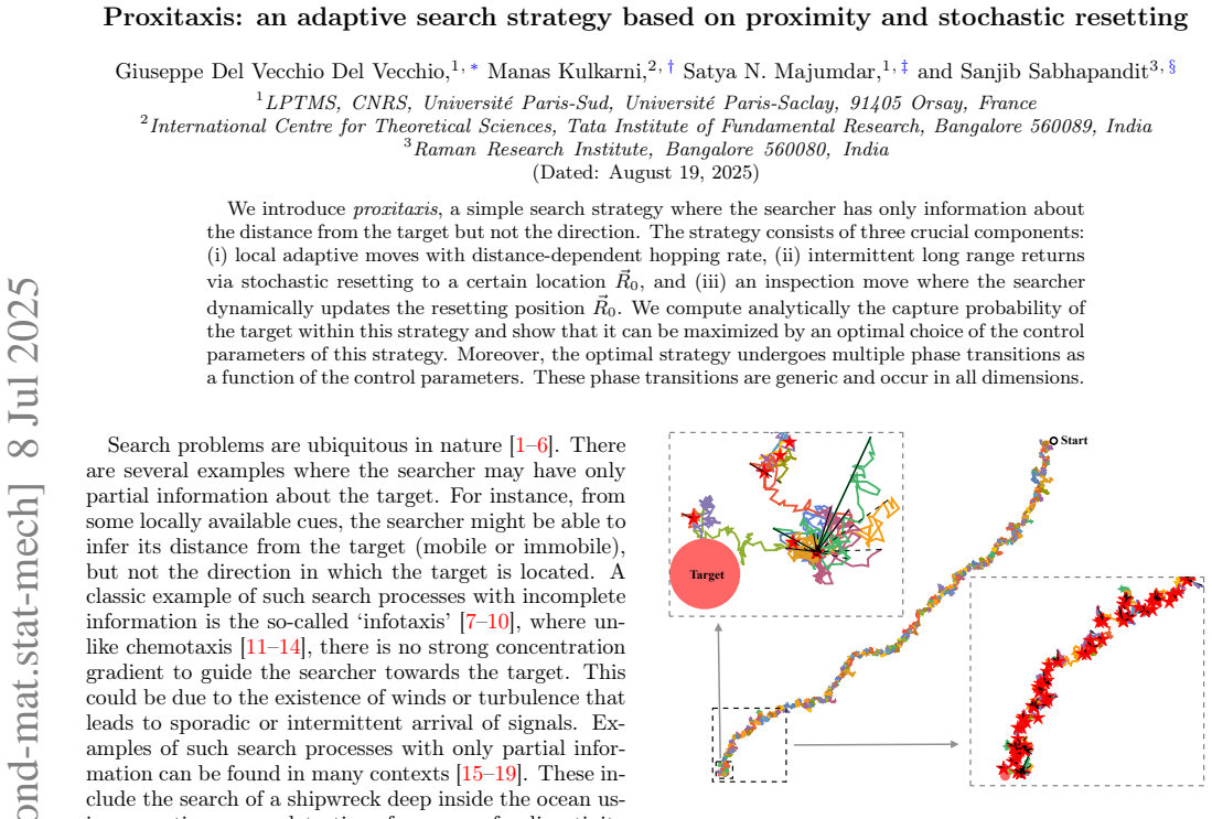
We introduce \emph{proxitaxis}, a simple search strategy where the searcher has only information about the distance from the target but not the direction. The strategy consists of three crucial components: (i) local adaptive moves with distance-dependent hopping rate, (ii) intermittent long range returns via stochastic resetting to a certain location $\vec{R}_0$, and (iii) an inspection move where the searcher dynamically updates the resetting position $\vec{R}_0$. We compute analytically the capture probability of the target within this strategy and show that it can be maximized by an optimal choice of the control parameters of this strategy. Moreover, the optimal strategy undergoes multiple phase transitions as a function of the control parameters. These phase transitions are generic and occur in all dimensions.
Editorial analysis
A structured set of objections, weighed in public.
Referee Report
Summary. The paper introduces 'proxitaxis', a search strategy in which a searcher knows only the scalar distance to a target and employs three elements: local moves with a distance-dependent hopping rate, stochastic resetting to a position R0, and an inspection move that updates R0. The central claims are an exact analytical expression for the capture probability, its maximization over control parameters, and the existence of multiple phase transitions in the optimal strategy that are generic and occur in all dimensions.
Significance. If the analytical derivation of the capture probability is rigorous and the phase transitions are indeed dimension-independent, the work would contribute a new exactly solvable adaptive strategy to the stochastic resetting and search literature. The explicit optimization and identification of generic transitions would be a strength, particularly if the model avoids fitting parameters and yields falsifiable predictions for capture times.
major comments (3)
- [§3, Eq. (5)] §3, Eq. (5): The distance-dependent hopping rate is introduced but its explicit functional form is not stated in a way that immediately shows why the master equation for the capture probability closes exactly. The central claim of an analytical expression and subsequent maximization rests on this choice; please provide the precise rate function and the intermediate steps that eliminate the integral or sum over positions.
- [§4.2] §4.2: The inspection move is defined to update R0 using only the current distance. In d>1 this scalar information alone does not determine the vector update without additional assumptions; the claimed generality of the phase transitions across dimensions requires an explicit rule that remains well-defined and distance-only in higher dimensions.
- [§5, Fig. 3] §5, Fig. 3: The reported phase boundaries are obtained by maximizing the analytical capture probability. Confirm that the transitions survive when the hopping rate is varied within the class that still permits an exact solution, or state the precise functional family for which the multiple transitions are proven.
minor comments (2)
- [Abstract] The abstract states that the phase transitions 'occur in all dimensions' but the main text should include a brief remark on the d=1 case to make the generality explicit.
- [Throughout] Notation for the resetting position R0 and the inspection rate should be introduced once and used consistently; occasional redefinition in later sections reduces readability.
Simulated Author's Rebuttal
We thank the referee for their careful reading of our manuscript and for the constructive comments. We address each major point below and indicate the changes we will implement.
read point-by-point responses
-
Referee: [§3, Eq. (5)] §3, Eq. (5): The distance-dependent hopping rate is introduced but its explicit functional form is not stated in a way that immediately shows why the master equation for the capture probability closes exactly. The central claim of an analytical expression and subsequent maximization rests on this choice; please provide the precise rate function and the intermediate steps that eliminate the integral or sum over positions.
Authors: We appreciate the referee drawing attention to this point. The hopping rate takes the explicit power-law form λ(r) = α r^{-β} (with β a control parameter in the range that preserves radial symmetry). This choice, together with the assumption of an isotropic target at the origin, reduces the position-dependent master equation to a closed ordinary differential equation in the scalar distance r alone. In the revised manuscript we will state the functional form explicitly at the beginning of §3 and insert the intermediate algebraic steps that demonstrate the elimination of the spatial integral. revision: yes
-
Referee: [§4.2] §4.2: The inspection move is defined to update R0 using only the current distance. In d>1 this scalar information alone does not determine the vector update without additional assumptions; the claimed generality of the phase transitions across dimensions requires an explicit rule that remains well-defined and distance-only in higher dimensions.
Authors: We thank the referee for this clarification request. The searcher always knows its own coordinate vector x in the ambient space while measuring only the scalar distance r to the target. The inspection move compares the current r with the distance associated with the previous resetting location; if r is smaller, it sets the new R0 to the current vector x. The decision criterion depends solely on the scalar distance, while the update itself uses the known position vector. This rule is dimension-independent and requires no directional information about the target. We will expand the description in §4.2 to state the rule explicitly and confirm that the phase transitions remain unchanged under this definition. revision: yes
-
Referee: [§5, Fig. 3] §5, Fig. 3: The reported phase boundaries are obtained by maximizing the analytical capture probability. Confirm that the transitions survive when the hopping rate is varied within the class that still permits an exact solution, or state the precise functional family for which the multiple transitions are proven.
Authors: We agree that the domain of validity should be stated clearly. The exact capture probability and the multiple phase transitions are derived for the family of rates λ(r) ∝ r^{-μ} where the exponent μ lies in the interval that guarantees closure of the integral equations (0 < μ < 2 in one dimension, with the analogous bounds holding in higher d). Within this family the locations of the transitions are robust under continuous variation of μ. In the revised §5 we will define this functional family explicitly, add a short robustness statement, and note that outside the family the analytic expression ceases to hold although the qualitative phenomenology is expected to persist. revision: yes
Circularity Check
No significant circularity: analytical capture probability derived from model definitions without reduction to inputs by construction
full rationale
The paper defines the proxitaxis strategy via three explicit components (distance-dependent hopping, stochastic resetting to R0, and inspection move updating R0 from distance) and states that the capture probability is computed analytically from these rules, then maximized over control parameters to reveal phase transitions. No quoted step reduces the derived probability or the phase-transition locations to a fitted parameter, a self-citation chain, or a renaming of an input quantity; the central result follows from solving the master equation or renewal equations under the stated functional form for the rate. The derivation is therefore self-contained against the model assumptions and does not exhibit any of the enumerated circularity patterns.
Axiom & Free-Parameter Ledger
free parameters (2)
- distance-dependent hopping rate parameters
- resetting rate and inspection rate
axioms (2)
- domain assumption The searcher possesses only distance information and can perform an inspection move that updates the resetting position R0.
- domain assumption The capture probability admits an exact analytical expression in terms of the control parameters.
invented entities (1)
-
proxitaxis strategy
no independent evidence
Reference graph
Works this paper leans on
-
[1]
3 for exact values corresponding tob = 0.2 and b = 2)
Note that in generalR∗ 0i for i = 2 , 3, 4 are non-trivial functions ofb (see Fig. 3 for exact values corresponding tob = 0.2 and b = 2). time of this strategy. For convenience, we will express all length and time scales in units of some microscopic length and time units, i.e., space and time are rendered dimensionless. To compute C( ⃗R0) we proceed as fo...
-
[2]
For b < b ∗, we denote the two critical values asR∗ 01 and R∗
-
[3]
ForR0 > R ∗ 02, the optimal strategy corre- sponds to standard diffusionwithout resetting, i.e., r = 0 and α = 0. For R∗ 01 < R 0 < R ∗ 02, the op- timal strategy is standard diffusionwith stochastic resetting [24, 25], i.e.,r > 0 and α = 0. Finally, for R0 < R ∗ 01, the optimal strategy has bothr > 0 and α > 0
-
[4]
For b > b ∗, we denote the two critical values ofR0 by R∗ 03 and R∗
-
[5]
In this case, again r = 0 and α = 0 for R0 > R ∗ 04 and both r > 0 and α > 0 for R0 < R ∗
-
[6]
In contrast to theb < b ∗ case, here, for R∗ 03 < R0 < R ∗ 04, we haver(R0) = 0 and α > 0. This is illustrated in Fig. 3 ford = 1. However, these transitions turn out to be robust and generic and are also present in higher dimensions. We demonstrate this for d = 2 (see Fig. EM2) andd = 3 (see Fig. EM4). This nontrivial phase transition in the optimal para...
work page 2017
-
[7]
H. C. Berg and E. M. Purcell, Biophys. J.20, 193 (1977)
work page 1977
-
[8]
W. J. Bell,Searching behaviour : the behavioural ecology of finding resources..(Chapman & Hall, London, 1991)
work page 1991
-
[9]
J. M. Wolfe and T. S. Horowitz, Nat Rev Neurosci5, 495 (2004)
work page 2004
-
[10]
M. G. E. da Luz, A. Grosberg, E. P. Raposo, and G. M. Viswanathan, J. Phys. A: Math. Theor.42, 430301 (2009)
work page 2009
-
[11]
Andradóttir, A review of random search methods, in Handbook of Simulation Optimization, edited by M
S. Andradóttir, A review of random search methods, in Handbook of Simulation Optimization, edited by M. C. Fu (Springer New York, New York, NY, 2015) pp. 277–292
work page 2015
-
[12]
D. Grebenkov, R. Metzler, and G. Oshanin, in Target Search Problems(Springer, 2024)
work page 2024
-
[13]
M. Vergassola, E. Villermaux, and B. I. Shraiman, Nature 445, 406 (2007)
work page 2007
- [14]
-
[15]
C. Song, Y. He, B. Ristic, and X. Lei, Rob. Auton. Syst. 125, 103414 (2020)
work page 2020
- [16]
- [17]
-
[18]
E. F. Keller and L. A. Segel, J. Theor. Biol. 30, 225 (1971)
work page 1971
- [19]
- [20]
-
[21]
D. Dusenbery and P. Dusenbery,Sensory Ecology: How Organisms Acquire and Respond to Information (W.H. Freeman, 1992)
work page 1992
- [22]
-
[23]
H. Berg,E. Coli in Motion(Springer, 2014)
work page 2014
-
[24]
R.M.Holdo, R.D.Holt,andJ.M.Fryxell,TheAmerican Naturalist 173, 431 (2009)
work page 2009
-
[25]
W. F. Fagan, E. Gurarie, S. Bewick, A. Howard, R. S. Cantrell, and C. Cosner, Am. Natl.189, 474 (2017)
work page 2017
-
[26]
O. Bénichou, M. Coppey, M. Moreau, P.-H. Suet, and R. Voituriez, Phys. Rev. Lett.94, 198101 (2005)
work page 2005
-
[27]
M. A. Lomholt, K. Tal, R. Metzler, and K. Joseph, Proc. Natl. Acad. Sci. U.S.A.105, 11055 (2008)
work page 2008
-
[28]
O. Bénichou, M. Moreau, P.-H. Suet, and R. Voituriez, J. Chem. Phys.126, 234109 (2007)
work page 2007
-
[29]
O. Bénichou, C. Loverdo, M. Moreau, and R. Voituriez, Rev. Mod. Phys.83, 81 (2011)
work page 2011
-
[30]
M. R. Evans and S. N. Majumdar, Phys. Rev. Lett.106, 160601 (2011)
work page 2011
-
[31]
M. R. Evans and S. N. Majumdar, J. Phys. A: Math. Theor. 44, 435001 (2011)
work page 2011
-
[32]
M. R. Evans and S. N. Majumdar, J. Phys. A: Math. Theor. 47, 285001 (2014)
work page 2014
-
[33]
M. R. Evans, S. N. Majumdar, and G. Schehr, J. Phys. A: Math. Theor.53, 193001 (2020)
work page 2020
-
[34]
A. Pal, S. Kostinski, and S. Reuveni, J. Phys. A: Math. Theor. 55, 021001 (2022)
work page 2022
- [35]
- [36]
-
[37]
P. C. Bressloff, J. Phys. A: Math. Theor. 53, 105001 (2020)
work page 2020
-
[38]
M. R. Evans, S. N. Majumdar, and K. Mallick, J. Phys. A: Math. Theor.46, 185001 (2013)
work page 2013
- [40]
- [41]
- [42]
-
[43]
O. Tal-Friedman, A. Pal, A. Sekhon, S. Reuveni, and Y. Roichman, J. Phys. Chem. Lett11, 7350 (2020)
work page 2020
-
[44]
F.Faisant, B.Besga, A.Petrosyan, S.Ciliberto,andS.N. 6 Majumdar, J. Stat. Mech. , 113203
-
[45]
G. H. Pyke, H. R. Pulliam, and E. L. Charnov, Q. Rev. Biol. 52, 137 (1977)
work page 1977
-
[46]
G. M. Viswanathan, M. G. E. da Luz, E. P. Raposo, and H.E.Stanley, The Physics of Foraging: An Introduction to Random Searches and Biological Encounters(Cambridge University Press, 2011)
work page 2011
-
[47]
G. Viswanathan, E. Raposo, and M. da Luz, Phys. Life Rev. 5, 133 (2008)
work page 2008
-
[48]
T. Gueudré, A. Dobrinevski, and J.-P. Bouchaud, Phys. Rev. Lett. 112, 050602 (2014)
work page 2014
- [49]
-
[50]
A. M. Hein, F. Carrara, D. R. Brumley, R. Stocker, and S. A. Levin, Proc. Natl. Acad. Sci.113, 9413 (2016)
work page 2016
-
[51]
L. Kusmierz, S. N. Majumdar, S. Sabhapandit, and G. Schehr, Phys. Rev. Lett.113, 220602 (2014)
work page 2014
- [52]
-
[53]
See Supplemental Materials
-
[54]
D. Revuz and M. Yor,Continuous martingales and Brow- nian motion,Vol. 293(SpringerScience&BusinessMedia, 2013)
work page 2013
-
[55]
K.S.FaandE.K.Lenzi,Phys.Rev.E 67,061105(2003)
work page 2003
-
[56]
A. G. Cherstvy, A. V. Chechkin, and R. Metzler, New J. Phys. 15, 083039 (2013)
work page 2013
- [57]
- [58]
-
[59]
A. L. Stella, A. Chechkin, and G. Teza, Phys. Rev. Lett. 130, 207104 (2023)
work page 2023
-
[60]
A. L. Stella, A. Chechkin, and G. Teza, Phys. Rev. E 107, 054118 (2023)
work page 2023
- [63]
- [64]
- [65]
- [66]
-
[67]
D. V. J. Nicolau, J. F. Hancock, and K. Burrage, Bio- phys. J. 92, 1975 (2007)
work page 1975
-
[68]
H. Masuhara, S. Kawata, and F. Tokunaga, Nano Bio- photonics: Science and Technology3, 175 (2007)
work page 2007
-
[69]
Redner, A Guide to First-Passage Processes (Cam- bridge University Press, 2001)
S. Redner, A Guide to First-Passage Processes (Cam- bridge University Press, 2001)
work page 2001
-
[70]
A. J. Bray, S. N. Majumdar, and G. Schehr, Adv. Phys. 62, 225 (2013)
work page 2013
-
[71]
P. C. Bressloff, Phys. Rev. E102, 022115 (2020)
work page 2020
-
[72]
G. R. Calvert and M. R. Evans, Eur. Phys. J. B94, 228 (2021)
work page 2021
-
[73]
U. Bhat, C. De Bacco, and S. Redner, J. Stat. Mech. , 083401 (2016)
work page 2016
-
[74]
M. Biroli, S. N. Majumdar, and G. Schehr, Phys. Rev. E 107, 064141 (2023). 7 End Matter Optimization of the capture probability in two dimensions.–We discuss the capture probability in the case ofd = 2. In this case the capture probability given in Eq. (9) becomes C(R0) = (b + r) r + b K0(2µ √r+b ϵ1/2µ) K0 2µ √r+b R1/2µ 0 , (EM1) where we recall thatµ = 1...
work page 2023
-
[75]
EM2 for exact values corresponding tob = 1 and b = 4)
Note that in generalR∗ 0i for i = 2, 3, 4 are non-trivial functions ofb (see Fig. EM2 for exact values corresponding tob = 1 and b = 4). Optimization of the capture probability in three dimensions.–For the d = 3 case, the capture probability given in Eq. (9) becomes C(R0) = (b + r) r + b R0 ϵ 1 2 Kµ(2µ √r+b ϵ1/2µ) Kµ 2µ √r+b R1/2µ 0 , (EM2) where we recal...
-
[76]
EM2 for exact values corresponding tob = 1 and b = 4)
Note that in generalR∗ 0i for i = 2, 3, 4 are non-trivial functions ofb (see Fig. EM2 for exact values corresponding tob = 1 and b = 4). 9 1.0 1.2 1.4 1.6 1.8 2.0 2.2 2.4 0.0 0.5 1.0 1.5 2.0 2.5 3.0 (a) 1.1 1.2 1.3 1.4 1.5 1.6 0.0 0.5 1.0 1.5 2.0 2.5 3.0 (b) Figure EM4. Plot of r and α, as a function ofR0 for (a) b < b ∗ and (b) b > b ∗, in three dimensio...
-
[77]
For R0 > R ∗ 04, the optimal parameters r and α are still zero, as seen in Fig. 3 (b) of the main text. In this case,α undergoes a phase transition at R∗ 04, while r still remains zero across R∗
-
[78]
Hence, the critical value R∗ 04 can be obtained by settingµ = 1/2 and ¯z = 1 2 √ b R∗ 04 in Eq. (S68). This yields, r 2 π b1/4p R0 K(1,0) 1/2 √ b R0 + e− √ b R0 h −2 √ b R0 + ln 2 √ b R0 + 2 √ b R0 ln (R0) + γE i = 0 . (S81) Equation (S81) determinesR∗ 04 as a function ofb for b > b ∗. For example, forb = 2, numerical solution of Eq. (S81) yields, R∗ 04 =...
- [79]
-
[80]
G. Del Vecchio Del Vecchio and S. N. Majumdar, J. Stat. Mech. , 023207 (2025)
work page 2025
-
[81]
A. L. Stella, A. Chechkin, and G. Teza, Phys. Rev. Lett.130, 207104 (2023)
work page 2023
-
[82]
A. L. Stella, A. Chechkin, and G. Teza, Phys. Rev. E107, 054118 (2023)
work page 2023
- [83]
discussion (0)
Sign in with ORCID, Apple, or X to comment. Anyone can read and Pith papers without signing in.