Multilayer GNN for Predictive Maintenance and Clustering in Power Grids

Chau Le; Harun Pirim; Muhammad Kazim; Om Prakash Yadav; Trung Le

REVIEW 4 major objections 4 minor 42 references

Multilayer GNN for Predictive Maintenance and Clustering in Power Grids

T0 review · 4 major / 4 minor · reviewed 2026-08-06 · deepseek-v4-flash

Challenge this review Re-run · record.json Download PDF Read on arXiv ↗

Pith's one-line read One GNN predicts grid failures and finds 8 risk clusters

desk verdict A competently built multilayer GNN clustering pipeline attached to a PdM claim that is undermined by a future-information label and a mismatched ablation quote. read the letter →

arxiv 2507.07298 v1 pith:TOM3CBHH submitted 2025-07-09 eess.SY cs.LGcs.SY

Muhammad Kazim , Harun Pirim , Chau Le , Trung Le , Om Prakash Yadav This is my paper · ORCID

classification eess.SYcs.LGcs.SY

keywords graphneuralnetworkspredictivemaintenancepowergridresiliencemultilayersubstationclusteringHDBSCANfailurepredictionspatial-temporal-causalmodeling

verification ladder T0 review T1 audit T2 compute T3 formal

The pith

A machine-rendered reading of the paper's core claim, the machinery that carries it, and where it could break.

The reading

This paper argues that power-grid predictive maintenance fails when substations are treated as isolated units, and that a multilayer graph neural network reasoning separately over spatial, temporal, and causal relationships can fix that. On seven years of Oklahoma Gas & Electric incident data, the proposed framework predicts which substations need major maintenance within 30 days with an F1-score of 0.8935 ± 0.0258, beating XGBoost and Random Forest by about three percentage points and single-layer GNNs by ten to fifteen. The same embeddings, clustered with HDBSCAN, separate the grid into eight operationally distinct risk groups, with one high-risk cluster showing roughly six times the incident rate of the safest clusters. The paper's central design claim is that the causal layer, built from statistically enriched co-occurrence of failures, carries most of the predictive power: removing it and using only spatial edges drops the F1-score to 0.7354 ± 0.0418.

What carries the argument

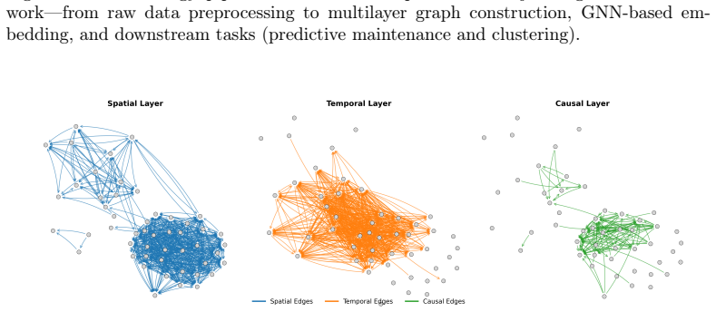
The machinery is a three-layer heterogeneous graph plus attention-weighted fusion. Spatial edges come from physical transmission lines and proximity-based links; temporal edges connect substations whose incidents fall within a data-driven 80th-percentile time window, weighted by exponential decay; causal edges are kept only when a cause-specific co-occurrence z-score exceeds the 85th percentile. Each layer is processed by its own GNN encoder—GATv2 for spatial and temporal, GIN for causal—and the per-layer embeddings are combined through a learned multi-head attention weight before a classifier head. The same fused embeddings feed UMAP plus HDBSCAN for clustering.

What would settle it

Retrain the same architecture with labels constructed from data available at prediction time—for example, define yi = 1 only from historical SAIDI and maintenance records with no look-ahead to the next incident—and compare the 30-day F1; a large drop would show the reported 0.8935 depends on future information rather than on the multilayer representation.

Watch

Extended reading notes

Core claim

The central claim is that modeling a power grid as a multilayer graph—with one edge layer for physical and geographic proximity, one for temporally co-occurring outages, and one for statistically enriched cause-specific failure co-occurrence—lets a single GNN architecture both forecast substation maintenance needs and recover meaningful resilience clusters. On the OGE dataset (292,830 records across 347 substations), the fused model reaches a 30-day F1-score of 0.8935 ± 0.0258, outperforming the classical baselines and single-layer GNN variants. Ablation shows the causal layer is the main driver, while the spatial layer alone performs worst. Clustering the learned embeddings yields eight risk groups whose separation is validated by ANOVA (p < 0.0001) and by operational metrics such as incidents per year and recovery time; the highest-risk cluster (44 substations) averages 388.4 incidents/year and 602.6 minutes recovery.

Load-bearing premise

The outcome label uses the time until the next severe failure (Δt_next > 180 days), which is only known after the fact; if a deployed model cannot see that future, the reported F1 scores may not reflect true forecasting skill.

Editorial extensions

If this is right

If the architecture holds, utilities can prioritize substations for maintenance with a single model that jointly uses physical, temporal, and causal relations instead of separate pipelines.
The causal layer's dominance suggests that co-failure statistics, not just distance or recency, are the most informative signal for predicting which substations need intervention.
The eight-cluster segmentation gives an operational zoning scheme: substations in Cluster 5 would be candidates for roughly six times more frequent inspection than Cluster 2, with weather-hardening and vegetation management focused there.
Because the framework's layers are modular, adding new relation types, such as cyber or market layers, could extend the same architecture to other infrastructure networks.

Reading between the lines

Editorial extensions of the paper, not claims the author makes directly.

The label's look-ahead means the headline F1 should be read as a ceiling; a fair prospective test would report performance when labels are frozen at training time and future failures are unknown.
The causal layer is not causal in the intervention sense; calling it 'causal' may overstate what correlation-enriched co-occurrence establishes, though it may still be a useful predictive signal.
The clustering's HDBSCAN parameters were tuned without ground truth, so the eight clusters are plausible but should be re-derived on a second utility's data before being used as a template.
A natural next test is to use the same embeddings to predict which failure cause will hit next, since the causal layer already encodes cause-specific windows and co-occurrence counts.

Share X Bluesky LinkedIn Reddit HN

Editorial analysis

A structured set of objections, weighed in public.

Desk editor's note, referee report, and a circularity audit.

Desk Editor's Note

read the letter

Two things you should know about arXiv:2507.07298. The headline PdM result — F1 0.8935 on a 30-day window — is computed against a label that uses future information. Section 2.4 defines yi = I[SAIDIi > Q90(SAIDI) and Δtnext > 180 days], where Δtnext is the time until the substation's next severe failure. At any real prediction time that quantity is unknown. The authors flag the assumption in Limitations, but the concession doesn't change the arithmetic; the F1 measures classification of a retrospectively constructed target, not forecasting skill. Second, the abstract and conclusion attribute the drop to 0.7354 to "removing the causal layer," but Table 4 shows 0.7354 is the spatial-only configuration. No spatial+temporal ablation is reported. The causal layer's marginal contribution is not quantified anywhere.

What is genuinely there: the paper assembles a real multilayer graph from 292,830 OGE incident records, with spatial, temporal, and causal edge types processed by separate GNN encoders (GATv2 and GIN) and fused with attention. That part is straightforward but competently done. The clustering pipeline — UMAP into three dimensions, HDBSCAN, eight clusters with interpretable risk profiles — is the more defensible contribution. The cluster statistics (incident rates, recovery times, ANOVA) are descriptively interesting, and the code/data link is provided. One caveat: the clustering embeddings are trained with MSE against historical incident frequencies, and the same frequencies are used to validate the clusters, so there's some circularity.

The evaluation protocol shifts between Section 2.5.3 (temporal split) and Section 3.1.1 (stratified 3-fold across substations), and neither removes the future-looking label. That inconsistency makes it hard to trust the variance estimates as well.

Who is this for? People working on GNNs for infrastructure analytics, and specifically anyone who wants a worked example of multilayer graph construction on utility outage data. The clustering results could inform maintenance planning if reproduced. But the PdM claim needs a corrected label definition — e.g., a fixed future horizon measured from the prediction point — and a genuinely reported ablation. As submitted, I'd reject, though I wouldn't desk-reject; the raw material is there. Send it to a referee, but expect heavy revision.

Referee Report

4 major / 4 minor

Summary. The paper proposes a multilayer graph neural network (GNN) framework for predictive maintenance (PdM) and resilience-based clustering of power-grid substations, applied to seven years of Oklahoma Gas & Electric incident data (292,830 records, 347 substations). Three edge layers (spatial, temporal, causal) are processed by GATv2, GATv2, and GIN encoders, fused via attention, and used for binary classification of substation maintenance needs and for HDBSCAN clustering on the learned embeddings. The authors report a 30-day F1-score of 0.8935, outperforming XGBoost and Random Forest by 3.2% and 2.7%, and single-layer GNN variants by 10–15%; they also report eight operational risk clusters with a Silhouette score of 0.626. The manuscript includes the code and data repository link and openly acknowledges limitations of the labeling strategy in the Limitations section.

Significance. If the reported results were valid, the framework would be a practically relevant contribution to predictive maintenance and risk-aware clustering in power grids. The paper has several strengths: it applies a multi-relational GNN architecture to a real utility dataset, provides code and data availability, and the clustering section attempts operational interpretation via incident rates, recovery times, and ANOVA-based risk differentiation. However, the central PdM claim rests on a label that incorporates future information, so the headline F1-score does not measure prospective forecasting skill. The ablation claim about the causal layer's marginal contribution is also not supported by the reported tables. Because the primary quantitative claims are undermined, the significance of the contribution as currently presented is low.

major comments (4)

[Section 2.4] The predictive maintenance label is defined as yi = I[SAIDIi > Q90(SAIDI) AND Δtnext > 180 days], where Δtnext is the time until the next severe failure at the same substation. This quantity is not observable at the time of prediction in any real deployment. The authors acknowledge this in the Limitations section ('assumes full temporal visibility'), but the acknowledgment does not repair the evaluation: training and test labels are constructed using post-cutoff incidents, so the reported F1-scores in Tables 1–3 and the headline 0.8935 (30-day window) measure classification of a retrospectively constructed target, not forecasting skill. The paper needs a prospective evaluation protocol where labels are defined only from information available up to the prediction time (e.g., a fixed cutoff, a subsequent observation window, and no condition on Δtnext). Without such a protocol, the central PdM claim is not valid.
[Abstract and Table 4] The abstract and conclusion state that 'removing the causal layer drops performance to 0.7354', but Table 4 reports 0.7354 for the 'Only Spatial Layer' configuration, which removes both the temporal and the causal layers. No 'spatial+temporal' ablation (i.e., removing only the causal layer) is reported. Consequently, the claimed marginal contribution of the causal layer is not quantified by the presented experiments; the 15% drop relative to the full model is attributable to the joint removal of two layers, not to the causal layer alone.
[Sections 2.6.1 and 3.2] The clustering validation is partly circular. The HierarchicalRiskGNN is trained with an MSE loss against historical incident frequencies for the four risk types (vegetation, weather, lightning, equipment) in Section 2.6.1, and the clusters are then validated using those same historical incident frequencies and recovery statistics in Tables 5 and 6 and Section 3.2.3. The ANOVA and reliability metrics therefore partly confirm that the embeddings preserve the training targets rather than discovering independent structure. To support the clustering claim, the authors should evaluate on held-out data or use an external validation metric not used in training, or clearly separate the training targets from the post-hoc operational metrics.
[Sections 2.5.3 and 3.1.1] The evaluation protocol is described inconsistently: Section 2.5.3 describes a temporal split (2015–2018 train, 2019 validation, 2020–2021 test), while Section 3.1.1 describes stratified 3-fold cross-validation across substations with per-fold target generation 'using only historical data up to the training cutoff'. These protocols have different leakage properties, and neither resolves the future-information problem in the label. The paper should specify the exact protocol used to produce Tables 1–3 and clarify how 'historical data up to the training cutoff' can be reconciled with the Δtnext condition in the label.

minor comments (4)

[Section 2.3] The node feature list is duplicated: the paragraph 'Node Features (V):' appears twice with identical content.
[Sections 2.6.2 and 3.2] The HDBSCAN cluster_selection_epsilon is stated as 0.5 in Section 2.6.2 and as 'epsilon=0.25' in Section 3.2; these values should be reconciled.
[Tables 1 and 4] The single-layer results (SPATIAL_ONLY, TEMPORAL_ONLY, CAUSAL_ONLY) appear in both Table 1 and the ablation Table 4, but the text does not clarify whether these are identical runs or re-evaluations; a clearer presentation would avoid confusion.
[Section 2.3.1] The spatial layer construction uses a 'confidence score' for fuzzy matching with thresholds 64 and 55–64, but the definition of this confidence score is not given; please cite the method or define it.

Circularity Check

3 steps flagged · score 6.0 of 10

Clustering validation reduces to training objectives: risk ANOVA, intra-cluster edge density, and Silhouette/DB all re-test the losses the HierarchicalRiskGNN was optimized on.

fitted input called prediction [Section 2.6.1 (HierarchicalRiskGNN training objective) and Section 3.2.2 (Risk Profile Differentiation)]
"Risk Prediction Loss: Predicts vegetation, weather, lightning, and equipment risk scores using MSE loss against historical incident frequencies. ... ANOVA tests across all clusters yielded statistically significant differentiation: Vegetation: F = 131.32, p = 0.0001 ... confirming that the observed differences in risk exposure across clusters are unlikely to have occurred by chance."

The ANOVA risk indicators are the exact historical frequencies used as supervision for the embedding: the model is trained to minimize MSE against vegetation, weather, lightning, and equipment incident counts, and the clusters are then cut in that embedding space. Finding that clusters differ on those same supervised targets is an in-sample check of the training objective, not an independent validation that clusters reflect risk. The operational-impact metrics (incidents/year, recovery time) are computed from the same raw outage records that supplied node features, so they partially re-import the same signal.
self definitional [Section 2.6.1 (Topological Consistency Loss) and Section 3.2.1 (Structural Validation)]
"Topological Consistency Loss: Encourages similar embeddings for directly connected nodes via cosine similarity objectives. ... observed intra-cluster ratios exceed random expectation and validate that the model learns meaningful structural patterns."

The structural-validation claim treats high intra-cluster edge density as emergent evidence that the model learned meaningful topology. But the embedding was explicitly trained with a Topological Consistency Loss that forces directly connected nodes to have similar embeddings; similar embeddings then tend to fall in the same HDBSCAN cluster. The reported intra-cluster edge ratios are therefore a direct consequence of the training objective, not an independent confirmation of structural learning.

1 more flagged steps

fitted input called prediction [Section 2.6.1 (Cluster Separation Loss) and Section 3.2.4 / Table 6 (Comparative Benchmarking)]
"Cluster Separation Loss: Encourages entropy-based separation and intra-cluster compactness using a deep clustering head. ... Our multilayer GNN-based clustering substantially outperforms the baselines: Cluster Cohesion: A Silhouette score of 0.626 reflects strong internal cohesion and well-separated clusters—nearly double that of KMeans (0.315)."

The model is trained with a Cluster Separation Loss that directly optimizes entropy-based separation and intra-cluster compactness. Reporting Silhouette and Davies-Bouldin as evidence of clustering quality—and benchmarking against KMeans and Spectral Clustering on the same optimized embeddings—evaluates the training objective itself. The superiority claimed for the GNN clustering is therefore partly built into the loss, not independently established.

full rationale

The PdM comparison is an ordinary supervised benchmark: Multi_GNN, Random Forest, and XGBoost all train on the same binary label, so their relative F1 differences are not circular by construction. However, the headline 30-day F1 (0.8935) is weakened by a future-information label: Section 2.4 defines yi = I[SAIDIi > Q90(SAIDI) and Delta_t_next > 180 days], where Delta_t_next is the time until the next severe failure and is not observable at prediction time; the authors concede this in Limitations ("assumes full temporal visibility"). I classify that as an evaluation-leakage/correctness risk rather than a derivation-equivalence circularity, so it does not by itself raise the circularity score, but it caps the strength of the forecasting claim. The clustering contributions are materially circular for the reasons in the three steps: the risk ANOVA, intra-cluster edge density, and Silhouette/DB index all validate objectives that were explicitly optimized when training the HierarchicalRiskGNN embeddings. The causal-layer ablation claim is also not supported as stated: the abstract says removing the causal layer drops F1 to 0.7354, but Table 4 shows 0.7354 for the spatial-only configuration, with no two-layer ablation isolating causal removal. The self-citations ([13], [15]) support background claims about multilayer energy networks but are not load-bearing for the main derivations. Overall, the predictive maintenance benchmarking has independent content, while the clustering 'validation' partially reduces to the training losses, giving a partial-circularity score of 6.

Assumptions & free parameters 8 free parameters · 6 assumptions · 0 invented entities

No new physical entities, forces, fields, dimensions, or conserved quantities are introduced. The causal layer is a statistical co-occurrence graph, and the paper explicitly disclaims formal causality in Section 2.3.3. The load-bearing assumptions are the fidelity of the incident logs, the Poisson co-occurrence model, the use of future information in labels, and the manual clustering parameters.

free parameters (8)

Temporal co-occurrence window θ = 80th percentile of global inter-incident intervals
Determines which incident pairs become temporal edges (Section 2.3.2); fitted to data.
Temporal edge co-occurrence filter k = max(3, median co-occurrence count)
Retains temporal edges with at least k occurrences; lower bound of 3 is empirical (Section 2.3.2).
Spatial proximity threshold = 75th percentile of distances among co-affected weather pairs
Creates proximity edges in the spatial layer (Section 2.3.1).
Causal edge enrichment thresholds = z-score at 85th percentile and observed count >= 3
Prunes the causal layer (Section 2.3.3).
PdM label thresholds = Q90(SAIDI) = 8.7 hours; Δtnext > 180 days
Defines yi in Section 2.4; the Δtnext term uses future incidents.
Focal loss parameters = α = 0.75, γ = 2
Training loss settings (Section 2.5.3).
Temporal edge decay constant = 60 minutes
Weight wt = exp(-|tu - tv|/60) for temporal edges (Section 2.3.2).
HDBSCAN clustering parameters = min_cluster_size = 15, min_samples = 5, epsilon = 0.5 (elsewhere 0.25)
Manual density-clustering settings (Sections 2.6.2, 3.2, and Limitations).

assumptions (6)

domain assumption Incident logs and fuzzy-matched substation identifiers faithfully represent the true failure process.
Preprocessing excludes unresolved records after Levenshtein matching with threshold 0.85 (Section 2.2.2).
domain assumption Co-occurrence enrichment with Poisson z-scores is a valid proxy for causal failure propagation.
Section 2.3.3 explicitly states this layer is not formal causal discovery, yet the ablation claim is framed as causal importance.
domain assumption The future gap Δtnext is observable when labels are assigned.
Section 2.4 defines yi using Δtnext > 180 days; Limitations admit this assumes full temporal visibility.
standard math Co-occurrence counts under independence follow a Poisson process with rate λu λv θc T.
Used to compute E[obs] and z-scores in Section 2.3.3.
domain assumption A single global percentile-based temporal window applies uniformly to all substations and causes.
θ is the global 80th percentile, not localized per node; the authors call it globally adaptive but not localized (Section 2.3.2).
domain assumption UMAP and HDBSCAN preserve meaningful cluster structure in the learned embedding space.
Used without formal guarantees; HDBSCAN parameters are manually tuned (Section 2.6.2, Limitations).

how reviews work

0 comments

Cite this review

Pith. "Pith review of Multilayer GNN for Predictive Maintenance and Clustering in Power Grids." pith.science (2026). https://pith.science/paper/TOM3CBHH

@misc{pith2026250707298,
  author       = {Pith},
  title        = {Pith review of: Multilayer GNN for Predictive Maintenance and Clustering in Power Grids},
  year         = {2026},
  howpublished = {\url{https://pith.science/paper/TOM3CBHH}},
  note         = {Machine review of arXiv:2507.07298}
}

abstract

Unplanned power outages cost the US economy over $150 billion annually, partly due to predictive maintenance (PdM) models that overlook spatial, temporal, and causal dependencies in grid failures. This study introduces a multilayer Graph Neural Network (GNN) framework to enhance PdM and enable resilience-based substation clustering. Using seven years of incident data from Oklahoma Gas & Electric (292,830 records across 347 substations), the framework integrates Graph Attention Networks (spatial), Graph Convolutional Networks (temporal), and Graph Isomorphism Networks (causal), fused through attention-weighted embeddings. Our model achieves a 30-day F1-score of 0.8935 +/- 0.0258, outperforming XGBoost and Random Forest by 3.2% and 2.7%, and single-layer GNNs by 10 to 15 percent. Removing the causal layer drops performance to 0.7354 +/- 0.0418. For resilience analysis, HDBSCAN clustering on HierarchicalRiskGNN embeddings identifies eight operational risk groups. The highest-risk cluster (Cluster 5, 44 substations) shows 388.4 incidents/year and 602.6-minute recovery time, while low-risk groups report fewer than 62 incidents/year. ANOVA (p < 0.0001) confirms significant inter-cluster separation. Our clustering outperforms K-Means and Spectral Clustering with a Silhouette Score of 0.626 and Davies-Bouldin index of 0.527. This work supports proactive grid management through improved failure prediction and risk-aware substation clustering.

Figures

Figures reproduced from arXiv: 2507.07298 by the authors.

**Figure 2.** Multilayer network architecture used in graph construction. Nodes repre [PITH_FULL_IMAGE:figures/full_fig_p007_2.png] view at source ↗

**Figure 3.** Incident cause distribution showing weather-related predominance [PITH_FULL_IMAGE:figures/full_fig_p008_3.png] view at source ↗

Figures from the paper (3 more)

**Figure 4.** Figure 4: Geospatial Distribution of Substation Clusters (HDBSCAN, 8 Clusters) [PITH_FULL_IMAGE:figures/full_fig_p026_4.png]

**Figure 5.** Figure 5: Distribution of Mean Recovery Time by Cluster. Clusters 5 and 3 exhibit [PITH_FULL_IMAGE:figures/full_fig_p027_5.png]

**Figure 6.** Figure 6: Cluster Impact Heatmap (Normalized). Cluster 5 stands out as the most oper [PITH_FULL_IMAGE:figures/full_fig_p028_6.png]

Discussion (0). Continue with ORCID to comment.

Reference graph

Works this paper leans on

42 extracted references · 31 canonical work pages

[1]

Available on- line: https://energycentral.com/news/fact-sheetbiden-harris (accessed: 2025-03-20)

The White House, FACT SHEET: Biden-Harris Administration An- nounces Investment to Bolster Electric Grid, 2023. Available on- line: https://energycentral.com/news/fact-sheetbiden-harris (accessed: 2025-03-20)

work page 2023
[2]

Department of Energy, Operations & maintenance best practices guide, release 3.0 (2010)

U.S. Department of Energy, Operations & maintenance best practices guide, release 3.0 (2010). URL:https://www.energy.gov/eere/femp/ operations-maintenance-best-practices-guide, accessed: 2025- 03-20

work page 2010
[3]

S.Geng, X.Wang, Predictivemaintenanceschedulingformultiplepower equipment based on data-driven fault prediction, Computers & Indus- trial Engineering 164 (2022) 107898

work page 2022
[4]

Schläpfer, S

M. Schläpfer, S. Dietz, M. Kaegi, Stress induced degradation dynamics in complex networks, in: 2008 First International Conference on Infras- tructure Systems and Services: Building Networks for a Brighter Future (INFRA), IEEE, 2008, pp. 1–5

work page 2008
[5]

B. Wu, A. Tang, J. Wu, Modeling cascading failures in interdependent infrastructuresunderterroristattacks, ReliabilityEngineering&System Safety 147 (2016) 1–8. 33

work page 2016
[6]

J. S. Jyoti, M. M. Hayat, Topological attributes of cascading failures in power grids, in: 2023 IEEE Power & Energy Society General Meeting (PESGM), IEEE, 2023, pp. 1–5

work page 2023
[7]

Cheng, Z

X. Cheng, Z. Zhang, Y. Bao, H. Zheng, Identification of high-risk sce- narios for cascading failures in new energy power grids based on deep embedding clustering algorithms., Energy Engineering 120 (2023)

work page 2023
[8]

B. Yu, H. Yin, Z. Zhu, Spatio-temporal graph convolutional net- works: A deep learning framework for traffic forecasting, arXiv preprint arXiv:1709.04875 (2018)

arXiv 2018

Show all 42 references

[9]

Z. Wu, S. Pan, G. Long, J. Jiang, C. Zhang, Graph wavenet for deep spatial-temporal graph modeling, arXiv preprint arXiv:1906.00121 (2019)

2019 arXiv
[10]

De Domenico, A

M. De Domenico, A. Solé-Ribalta, E. Cozzo, M. Kivelä, Y. Moreno, M. A. Porter, S. Gómez, A. Arenas, Mathematical formulation of mul- tilayer networks, Physical Review X 3 (2013) 041022

2013
[11]

Nicosia, V

V. Nicosia, V. Latora, Measuring and modeling correlations in multi- plex networks, Physical Review E 92 (2015) 032805. URL:https:// doi.org/10.1103/PhysRevE.92.032805. doi: 10.1103/PhysRevE.92. 032805

2015 doi
[12]

M. G. Puxeddu, M. Petti, L. Astolfi, A comprehensive analysis of multi- layer community detection algorithms for application to eeg-based brain networks, Frontiers in systems neuroscience 15 (2021) 624183

2021
[13]

Kazim, H

M. Kazim, H. Pirim, C. Le, T. Le, O. P. Yadav, Link prediction and nav- igability of multiplex energy networks, arXiv preprint arXiv:2503.14641 (2025)

2025 arXiv
[14]

Nosyreva, L

E. Nosyreva, L. Massel, Application of multilayer networks to detect criticalenergyfacilities, in: VIthInternationalWorkshop’CriticalInfras- tructures: Contingency Management, Intelligent, Agent-Based, Cloud Computing and Cyber Security’(IWCI 2019), Atlantis Press, 2019, pp. 249–256

2019
[15]

Kazim, H

M. Kazim, H. Pirim, S. Shi, D. Wu, Multilayer analysis of energy net- works, Sustainable Energy, Grids and Networks 39 (2024) 101407. 34

2024
[16]

Zhang, P

Y. Zhang, P. M. Karve, S. Mahadevan, Graph neural networks for power grid operational risk assessment under evolving grid topol- ogy, arXiv preprint arXiv:2405.07343 (2024).https://arxiv.org/abs/ 2405.07343

2024 arXiv
[17]

Ifeanyi, A graph neural network approach to system-level health index and remaining useful life estimation, Annual Conference of the PHM Society 16 (2024)

A. Ifeanyi, A graph neural network approach to system-level health index and remaining useful life estimation, Annual Conference of the PHM Society 16 (2024). URL:https://doi.org/10.36001/phmconf. 2024.v16i1.4159. doi:10.36001/phmconf.2024.v16i1.4159

2024 doi
[18]

M. A. Islam, M. Ismail, O. Boyaci, R. Atat, S. Shannigrahi, Graph neural network based prediction of data traffic in cyber-physical smart power grids, in: 2022 IEEE International Conference on Communica- tions, Control, and Computing Technologies for Smart Grids (Smart- GridCo...

2022
[19]

L. Xia, P. Zheng, X. Li, R. X. Gao, L. Wang, Toward cognitive pre- dictive maintenance: A survey of graph-based approaches, Journal of Manufacturing Systems 64 (2022) 107–120

2022
[20]

Grassia, M

M. Grassia, M. De Domenico, G. Mangioni, mgnn: Generalizing the graph neural networks to the multilayer case, arXiv preprint arXiv:2109.10119 (2021)

2021 arXiv
[21]

Ghorbani, M

M. Ghorbani, M. S. Baghshah, H. R. Rabiee, Mgcn: Semi-supervised classification in multi-layer graphs with graph convolutional networks, in: Proceedingsofthe2019IEEE/ACMInternationalConferenceonAd- vancesinSocialNetworksAnalysisandMining, 2019, pp.208–215.URL: https://doi.org/...

2019
[22]

Meng, et al., Deepmcgcn: Multi-channel deep graph neural networks, International Journal of Computational Intelligence Systems 17 (2024) 41

L. Meng, et al., Deepmcgcn: Multi-channel deep graph neural networks, International Journal of Computational Intelligence Systems 17 (2024) 41

2024
[23]

Q. Li, J. Li, L. Wang, C. Ji, Y. Hei, J. Sheng, Q. Sun, S. Xue, P. Xie, Type information utilized event detection via multi-channel gnns in elec- trical power systems, ACM Transactions on the Web 17 (2023) 1–26. 35

2023
[24]

Zhang, J

Z. Zhang, J. Li, Y. Wang, W. Liu, H. Zhang, Interpretable multi-graph convolution network integrating spatio-temporal correlations for wind power forecasting, Expert Systems with Applications 212 (2024) 124766. URL: https://doi.org/10.1016/j.eswa.2024.124766. doi:10.1016/ j.es...

2024
[25]

Huang, D

X. Huang, D. Chen, T. Ren, D. Wang, A survey of community de- tection methods in multilayer networks, Data Mining and Knowl- edge Discovery 35 (2021) 1–45. URL: https://doi.org/10.1007/ s10618-020-00716-6. doi:10.1007/s10618-020-00716-6

2021 doi
[26]

Amini Badr, A

A. Amini Badr, A. Safari, S. Najafi Ravadanegh, Segmentation of interconnected power systems considering microgrids and the uncer- tainty of renewable energy sources, IET Generation, Transmission & Distribution 17 (2023) 3814–3827. URL: https://ietresearch. onlinelibrary.wiley...

2023 doi
[27]

Losapio, D

G. Losapio, D. Beretta, M. Mussi, A. M. Metelli, M. Restelli, State and action factorization in power grids, arXiv preprint arXiv:2409.04467 (2024). https://arxiv.org/abs/2409.04467

2024 arXiv
[28]

Y. Zhao, H. Liao, S. Pan, Y. Zhao, Interpretable multi-graph convolu- tion network integrating spatio-temporal attention and dynamic combi- nation for wind power forecasting, Expert Systems with Applications 255 (2024) 124766

2024
[29]

V. I. Levenshtein, et al., Binary codes capable of correcting deletions, insertions, and reversals, in: Soviet physics doklady, volume 10, Soviet Union, 1966, pp. 707–710

1966
[30]

M. B. Araújo, A. Rozenfeld, C. Rahbek, P. A. Marquet, Using co- occurrence information to infer species interactions: a new approach, Ecography 34 (2011) 186–193

2011
[31]

Pearl, Causality, Cambridge University Press, 2009

J. Pearl, Causality, Cambridge University Press, 2009

2009
[32]

T.-Y. Lin, P. Goyal, R. Girshick, K. He, P. Dollár, Focal loss for dense object detection, in: Proceedings of the IEEE International Conference on Computer Vision (ICCV), 2017, pp. 2980–2988. 36

2017
[33]

Brody, E

S. Brody, E. Yahav, L. Barak, How attentive are graph attention networks?, in: International Conference on Learning Representations (ICLR), 2022

2022
[34]

K. Xu, W. Hu, J. Leskovec, S. Jegelka, How powerful are graph neural networks?, in: International Conference on Learning Representations (ICLR), 2019

2019
[35]

Loshchilov, F

I. Loshchilov, F. Hutter, Decoupled weight decay regularization, arXiv preprint arXiv:1711.05101 (2017)

2017 arXiv
[36]

McInnes, J

L. McInnes, J. Healy, J. Melville, Umap: Uniform manifold ap- proximation and projection for dimension reduction, arXiv preprint arXiv:1802.03426 (2018)

2018 arXiv
[37]

R. J. Campello, D. Moulavi, J. Sander, A density-based algorithm for discovering clusters in large spatial databases with noise, Advances in Knowledge Discovery and Data Mining (PAKDD) (2013) 160–172

2013
[38]

E. L. Kaplan, P. Meier, Nonparametric estimation from incomplete observations, Journal of the American Statistical Association 53 (1958) 457–481

1958
[39]

Breiman, Random forests, Machine learning 45 (2001) 5–32

L. Breiman, Random forests, Machine learning 45 (2001) 5–32

2001
[40]

T. Chen, C. Guestrin, Xgboost: A scalable tree boosting system, in: Proceedings of the 22nd acm sigkdd international conference on knowl- edge discovery and data mining, 2016, pp. 785–794

2016
[41]

P. J. Rousseeuw, Silhouettes: a graphical aid to the interpretation and validation of cluster analysis, Journal of computational and applied mathematics 20 (1987) 53–65

1987
[42]

A. Y. Ng, M. I. Jordan, Y. Weiss, On spectral clustering: Analysis and an algorithm, in: Advances in neural information processing systems, 2002, pp. 849–856. 37

2002

Pith tools

Reviewed August 6, 2026 · model on record in the stance chip above.

[1] [1]

Available on- line: https://energycentral.com/news/fact-sheetbiden-harris (accessed: 2025-03-20)

The White House, FACT SHEET: Biden-Harris Administration An- nounces Investment to Bolster Electric Grid, 2023. Available on- line: https://energycentral.com/news/fact-sheetbiden-harris (accessed: 2025-03-20)

work page 2023

[2] [2]

Department of Energy, Operations & maintenance best practices guide, release 3.0 (2010)

U.S. Department of Energy, Operations & maintenance best practices guide, release 3.0 (2010). URL:https://www.energy.gov/eere/femp/ operations-maintenance-best-practices-guide, accessed: 2025- 03-20

work page 2010

[3] [3]

S.Geng, X.Wang, Predictivemaintenanceschedulingformultiplepower equipment based on data-driven fault prediction, Computers & Indus- trial Engineering 164 (2022) 107898

work page 2022

[4] [4]

Schläpfer, S

M. Schläpfer, S. Dietz, M. Kaegi, Stress induced degradation dynamics in complex networks, in: 2008 First International Conference on Infras- tructure Systems and Services: Building Networks for a Brighter Future (INFRA), IEEE, 2008, pp. 1–5

work page 2008

[5] [5]

B. Wu, A. Tang, J. Wu, Modeling cascading failures in interdependent infrastructuresunderterroristattacks, ReliabilityEngineering&System Safety 147 (2016) 1–8. 33

work page 2016

[6] [6]

J. S. Jyoti, M. M. Hayat, Topological attributes of cascading failures in power grids, in: 2023 IEEE Power & Energy Society General Meeting (PESGM), IEEE, 2023, pp. 1–5

work page 2023

[7] [7]

Cheng, Z

X. Cheng, Z. Zhang, Y. Bao, H. Zheng, Identification of high-risk sce- narios for cascading failures in new energy power grids based on deep embedding clustering algorithms., Energy Engineering 120 (2023)

work page 2023

[8] [8]

B. Yu, H. Yin, Z. Zhu, Spatio-temporal graph convolutional net- works: A deep learning framework for traffic forecasting, arXiv preprint arXiv:1709.04875 (2018)

arXiv 2018