REVIEW 3 major objections 6 minor 22 references
GRIT: Graph Transformer For Internal Ice Layer Thickness Prediction
T0 review · 3 major / 6 minor · reviewed 2026-08-06 · deepseek-v4-flash
Pith's one-line read GRIT predicts thickness of 15 deeper Greenland ice layers from 5 shallow layers with mean RMSE 3.06 m, beating four graph-network baselines.
desk verdict GRIT is a sensible but incremental graph-transformer adaptation for ice-layer prediction; the evaluation as reported does not isolate the architecture, so the claimed advantage is not established. read the letter →
The pith
A machine-rendered reading of the paper's core claim, the machinery that carries it, and where it could break.
The reading
What carries the argument
The load-bearing component is the temporal multi-head attention block, adapted from the standard transformer encoder and applied along the temporal dimension of the GraphSAGE embeddings. Each input layer is a spatial graph of 256 nodes whose edge weights are inverse geographic distances computed with the haversine formula and whose node features are latitude, longitude, and layer thickness; five independent GraphSAGE encoders produce feature embeddings that are then attended over with eight heads using scaled dot-product attention. The attention mechanism is what lets the model weigh all shallow layers jointly and capture dependencies that recurrent graph networks would have to propagate step by step.
What would settle it
A fair comparison experiment would retrain every baseline and GRIT with the identical learning-rate schedule and initial learning rate on the same five data splits. If GRIT's mean RMSE is no longer below the Multi-branch baseline, the claim that the temporal attention block drives the improvement is falsified; an ablation that removes the attention block from GRIT while keeping everything else fixed would give the same answer.
Extended reading notes
Core claim
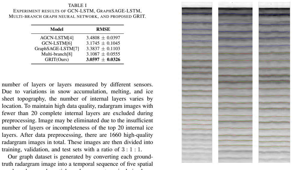
GRIT's central claim is that long-range temporal dependencies across ice layers are better learned by a transformer's multi-head attention than by the recurrent aggregation used in prior graph networks. The network encodes each of the five input layers with an independent GraphSAGE block, concatenates the spatial embeddings, and runs them through an 8-head temporal attention encoder before a two-layer convolutional decoder produces the 15 target thickness maps. On the CReSIS Greenland 2012 dataset, GRIT achieves a mean RMSE of 3.0597 ± 0.0326 m across five shuffled train/validation/test splits, the lowest among AGCN-LSTM (3.4808 ± 0.0397), GCN-LSTM (3.1745 ± 0.1045), GraphSAGE-LSTM (3.3837 ± 0.1103), and Multi-branch (3.1087 ± 0.0555). The paper also reports lower standard deviation, which it reads as more stable predictions.
Load-bearing premise
The reported advantage assumes GRIT and the baselines are compared fairly; because GRIT is trained with an adaptive learning-rate schedule starting at 0.001 while every baseline uses a step decay starting at 0.01, the lower RMSE could come from better tuning rather than from the temporal attention block.
Editorial extensions
If this is right
- GRIT predicts the thickness of 15 deeper internal ice layers from the top 5 layers with a mean RMSE of 3.0597 ± 0.0326 m on the CReSIS Greenland 2012 dataset.
- The temporal attention block yields consistently lower prediction error and lower variance than recurrent graph convolutional baselines, indicating attention can replace recurrent temporal modeling in this task.
- The architecture is designed to generalize to any number of input and output layers and to radargrams of different sizes, so the same network can be repurposed for other depth ranges or sensors.
- Because GRIT uses an inductive GraphSAGE encoder, it can produce embeddings for nodes not seen during training, which matters for new flight lines over the ice sheet.
Reading between the lines
- Editorial extension: the reported comparison does not rule out that GRIT's lower error comes from its adaptive learning-rate schedule (initial 0.001) versus the baselines' step decay (initial 0.01); a matched-schedule rerun would isolate the attention block's contribution.
- Editorial extension: attention weights could be inspected to identify which shallow years carry the most information about a given deep layer, turning the model from a predictor into a diagnostic of snow accumulation history.
- Editorial extension: because the graph representation is built only from coordinates and thickness, the same GRIT design could ingest other continuous fields measured along flight lines, such as radar echo strength or surface elevation, without changing the architecture.
Editorial analysis
A structured set of objections, weighed in public.
Referee Report
Summary. The paper introduces GRIT, a graph transformer for predicting the thickness of deep internal ice layers from shallow layers. The architecture uses five GraphSAGE encoders to produce spatial node embeddings for each of the m=5 input layers, a temporal multi-head attention block to model dependencies across layers, and two convolutional layers as a decoder to predict n=15 output layers. On the CReSIS Greenland 2012 dataset, the authors report a mean RMSE of 3.0597 ± 0.0326 m over five data-split permutations, which is lower than the reported RMSEs of four recurrent graph-convolutional baselines (best baseline: multi-branch GNN, 3.1087 ± 0.0555 m). The paper claims the attention mechanism is effective for capturing temporal changes, but the experimental protocol does not fully support this attribution because the training schedules are not matched and no significance test or ablation is provided.
Significance. If the claimed improvement is robust, GRIT represents a useful step for automated ice-layer thickness estimation from airborne radar, an important task for climate modeling. The paper has strengths: it uses real CReSIS data, describes data preprocessing clearly, and evaluates across five random train/validation/test splits, which is more careful than many short conference papers. However, the practical significance of the reported gain is uncertain: the mean RMSE difference to the best baseline (0.049 m) is smaller than the baseline's standard deviation (0.0555 m), and the unmatched optimization schedules prevent the conclusion that the architecture, rather than hyperparameter choice, drives the result. The central claim is plausible but not yet established at the level required for a definitive journal publication; the missing matched-schedule comparison and ablation are the key gaps.
major comments (3)
- [Section V-B; Table I] The optimization protocol is not matched between GRIT and the baselines. GRIT is trained with an adaptive learning-rate scheduler (initial learning rate 0.001, halving after 16 epochs without validation improvement), while all baselines use a step scheduler (initial learning rate 0.01, halving every 75 epochs). Since learning-rate schedules strongly affect the final RMSE of recurrent GNNs, this setup confounds model architecture with training recipe. The reported advantage over the best baseline, 3.1087 - 3.0597 = 0.049 m, is smaller than the standard deviation of that baseline (0.0555 m) and no paired significance test is reported. I request a matched-schedule comparison (e.g., train all models with the same scheduler or include a grid of initial learning rates) and per-split RMSE values with a paired significance test (e.g., Wilcoxon signed-rank test).
- [Section V-C; Figure 2; Conclusion] The paper attributes GRIT's lower error to the temporal attention block ('these results highlight the attention mechanism's effectiveness'), but no ablation study supports this attribution. To isolate the contribution of temporal attention, please add an ablation that replaces the temporal multi-head attention block with a recurrent layer (e.g., an LSTM) or removes it entirely, while keeping the GraphSAGE encoders, the decoder, and the training schedule fixed. Without such an ablation, the architecture's advantage could stem from any other component (e.g., the number of parameters or the inductive GraphSAGE encoders).
- [Section V-A, Eq. (5)] Equation (5) does not correctly state the inverse-distance edge weight. The haversine distance is normally \(2R\arcsin(\sqrt{\mathrm{hav}(\phi_j-\phi_i)+\cos\phi_i\cos\phi_j\,\mathrm{hav}(\lambda_j-\lambda_i)})\), and the edge weight should be the reciprocal of that distance. As written, the formula omits the square root and the Earth's radius and sets the weight to the reciprocal of the arcsin term, which is dimensionally and numerically inconsistent. Please correct the formula or clarify the exact computation used for the graph edge weights.
minor comments (6)
- [Section V heading] The heading 'EXPERIEMENTS' should be 'EXPERIMENTS'.
- [Section III] 'CRsSIS' should be 'CReSIS'.
- [Section I, Introduction] The acronym definition 'Graph t Ransfromer from For Ice layer Thickness' contains a typo; it should be 'Graph Transformer for Ice Layer Thickness'.
- [References] References [2] and [18] are duplicate entries for the same Gogineni et al. paper; please merge or renumber.
- [Section V-B] The paper does not report model parameter counts or training time, which makes it difficult to assess whether GRIT's improvement is due to increased model capacity; please add these details.
- [Figure 1] The architecture diagram in Figure 1 is difficult to read at print resolution; please increase the font size or split it into clearly labeled subfigures.
Circularity Check
No significant circularity: GRIT's claimed performance is an empirical benchmark on held-out test splits, not a quantity defined by its inputs.
full rationale
The paper's derivation chain is a supervised learning pipeline: five GraphSAGE encoders produce spatial embeddings, a multi-head temporal attention block transforms the temporal dimension, and a convolutional decoder outputs thickness values for the 15 deeper layers; the model is trained with MSE loss on disjoint image splits and evaluated by RMSE on held-out test sets. Nothing in the equations or dataset construction defines the reported 3.0597 m RMSE in terms of the inputs or a fitted parameter renamed as a prediction. The baselines are prior works from the same research group, but the paper states that all networks were retrained on the same machine with the same number of epochs and five random data permutations, so Table I is not a citation-based assertion of superiority. The main legitimate concern is a training-protocol confound (GRIT uses an adaptive learning-rate scheduler starting at 0.001, while every baseline uses a step scheduler starting at 0.01) and the absence of an ablation isolating the temporal attention block; those are correctness and rigor issues, not circularity, because the reported numbers are still empirical outcomes. No load-bearing argument in the paper reduces to a self-citation or a definitional equivalence.
Assumptions & free parameters
free parameters (6)
- Number of input ice layers m =
5
- Number of output ice layers n =
15
- Number of nodes per spatial graph =
256
- Number of attention heads =
8
- Initial learning rate for GRIT =
0.001
- Training epochs =
450
assumptions (5)
- domain assumption Manually labeled ice layer boundaries by NASA scientists are accurate enough to serve as ground truth.
- domain assumption A 256-node graph per layer with inverse haversine edge weights captures the spatial structure of the ice layer.
- domain assumption Thickness values of the top 5 layers are predictive of the thickness of the next 15 layers.
- domain assumption The five random dataset permutations provide a meaningful estimate of model performance variability.
- domain assumption The edge weight formula in Eq. 5 is a correct distance measure.
Cite this review
Pith. "Pith review of GRIT: Graph Transformer For Internal Ice Layer Thickness Prediction." pith.science (2026). https://pith.science/paper/46QJRKJQ
@misc{pith2026250707388,
  author       = {Pith},
  title        = {Pith review of: GRIT: Graph Transformer For Internal Ice Layer Thickness Prediction},
  year         = {2026},
  howpublished = {\url{https://pith.science/paper/46QJRKJQ}},
  note         = {Machine review of arXiv:2507.07388}
}
read the original abstract
Gaining a deeper understanding of the thickness and variability of internal ice layers in Radar imagery is essential in monitoring the snow accumulation, better evaluating ice dynamics processes, and minimizing uncertainties in climate models. Radar sensors, capable of penetrating ice, capture detailed radargram images of internal ice layers. In this work, we introduce GRIT, graph transformer for ice layer thickness. GRIT integrates an inductive geometric graph learning framework with an attention mechanism, designed to map the relationships between shallow and deeper ice layers. Compared to baseline graph neural networks, GRIT demonstrates consistently lower prediction errors. These results highlight the attention mechanism's effectiveness in capturing temporal changes across ice layers, while the graph transformer combines the strengths of transformers for learning long-range dependencies with graph neural networks for capturing spatial patterns, enabling robust modeling of complex spatiotemporal dynamics.
Figures

Reference graph
Works this paper leans on
-
[1]
Chapter 12 - glaciers and ice sheets,
S. A. Arcone, “Chapter 12 - glaciers and ice sheets,” in Ground Penetrating Radar Theory and Applications , H. M. Jol, Ed. Amsterdam: Elsevier, 2009, pp. 361–392. [Online]. Available: https://www.sciencedirect.com/science/ article/pii/B9780444533487000120
work page 2009
-
[3]
Cresis airborne radars and platforms for ice and snow sounding,
E. Arnold, C. Leuschen, F. Rodriguez-Morales, J. Li, J. Paden, R. Hale, and S. Keshmiri, “Cresis airborne radars and platforms for ice and snow sounding,” Annals of Glaciology , vol. 61, no. 81, p. 58–67, 2020
work page 2020
-
[4]
Prediction of deep ice layer thickness using adaptive recurrent graph neural networks,
B. Zalatan and M. Rahnemoonfar, “Prediction of deep ice layer thickness using adaptive recurrent graph neural networks,” in 2023 IEEE International Conference on Image Processing (ICIP), 2023, pp. 2835–2839
work page 2023
-
[5]
Prediction of annual snow accumulation using a recur- rent graph convolutional approach,
——, “Prediction of annual snow accumulation using a recur- rent graph convolutional approach,” in IGARSS 2023 - 2023 IEEE International Geoscience and Remote Sensing Sympo- sium, 2023, pp. 5344–5347
work page 2023
-
[6]
——, “Recurrent graph convolutional networks for spatiotem- poral prediction of snow accumulation using airborne radar,” in 2023 IEEE Radar Conference (RadarConf23) , 2023, pp. 1–6
work page 2023
-
[7]
Learning spatio-temporal patterns of polar ice layers with physics-informed graph neural network,
Z. Liu and M. Rahnemoonfar, “Learning spatio-temporal patterns of polar ice layers with physics-informed graph neural network,” 2024. [Online]. Available: https://arxiv.org/abs/2406. 15299
work page 2024
-
[8]
Multi-branch spatio-temporal graph neural network for efficient ice layer thickness prediction,
——, “Multi-branch spatio-temporal graph neural network for efficient ice layer thickness prediction,” 2024. [Online]. Available: https://arxiv.org/abs/2411.04055
arXiv 2024
-
[9]
Physics-informed machine learning for deep ice layer tracing in sar images,
M. Rahnemoonfar and B. Zalatan, “Physics-informed machine learning for deep ice layer tracing in sar images,” in IGARSS 2024 - 2024 IEEE International Geoscience and Remote Sens- ing Symposium , 2024, pp. 6938–6942
work page 2024
Show all 22 references
-
[10]
Learning snow layer thickness through physics defined labels,
D. Varshney, O. Ibikunle, J. Paden, and M. Rahnemoonfar, “Learning snow layer thickness through physics defined labels,” in IGARSS 2022 - 2022 IEEE International Geoscience and Remote Sensing Symposium , 2022, pp. 1233–1236
2022
-
[11]
Deep ice layer tracking and thickness estimation using fully convo- lutional networks,
D. Varshney, M. Rahnemoonfar, M. Yari, and J. Paden, “Deep ice layer tracking and thickness estimation using fully convo- lutional networks,” in 2020 IEEE International Conference on Big Data (Big Data) , 2020, pp. 3943–3952
2020
-
[12]
Deep learning on airborne radar echograms for tracing snow accumulation layers of the greenland ice sheet,
D. Varshney, M. Rahnemoonfar, M. Yari, J. Paden, O. Ibikunle, and J. Li, “Deep learning on airborne radar echograms for tracing snow accumulation layers of the greenland ice sheet,” Remote Sensing , vol. 13, no. 14, 2021. [Online]. Available: https://www.mdpi.com/2072-4292/13/14/2707
2021
-
[13]
Deep multi-scale learning for automatic tracking of internal layers of ice in radar data,
M. Rahnemoonfar, M. Yari, J. Paden, L. Koenig, and O. Ibikunle, “Deep multi-scale learning for automatic tracking of internal layers of ice in radar data,” Journal of Glaciology , vol. 67, no. 261, p. 39–48, 2021
2021
-
[14]
Airborne snow radar data simulation with deep learning and physics-driven methods,
M. Yari, O. Ibikunle, D. Varshney, T. Chowdhury, A. Sarkar, J. Paden, J. Li, and M. Rahnemoonfar, “Airborne snow radar data simulation with deep learning and physics-driven methods,” IEEE Journal of Selected Topics in Applied Earth Observations and Remote Sensing , vol. 14, pp...
2021
-
[15]
Deep hybrid wavelet network for ice boundary de- tection in radra imagery,
H. Kamangir, M. Rahnemoonfar, D. Dobbs, J. Paden, and G. Fox, “Deep hybrid wavelet network for ice boundary de- tection in radra imagery,” in IGARSS 2018 - 2018 IEEE Inter- national Geoscience and Remote Sensing Symposium , 2018, pp. 3449–3452
2018
-
[16]
Refining ice layer tracking through wavelet combined neural networks,
D. Varshney, M. Yari, T. Chowdhury, and M. Rahnemoonfar, “Refining ice layer tracking through wavelet combined neural networks,” in ICML 2021 Workshop on Tackling Climate Change with Machine Learning , 2021. [Online]. Available: https://www.climatechange.ai/papers/icml2021/49
2021
-
[17]
Evolvegcn: Evolving graph convolutional networks for dynamic graphs,
A. Pareja, G. Domeniconi, J. Chen, T. Ma, T. Suzumura, H. Kanezashi, T. Kaler, and C. E. Leiserson, “Evolvegcn: Evolving graph convolutional networks for dynamic graphs,” CoRR, vol. abs/1902.10191, 2019. [Online]. Available: http: //arxiv.org/abs/1902.10191
1902 arXiv
-
[18]
Ultra-wideband radars for remote sensing of snow and ice,
S. Gogineni, J. B. Yan, D. Gomez, F. Rodriguez-Morales, J. Paden, and C. Leuschen, “Ultra-wideband radars for remote sensing of snow and ice,” in IEEE MTT-S International Mi- crowave and RF Conference , 2013, pp. 1–4
2013
-
[19]
Icebridge snow radar l1b geolocated radar echo strength profiles,
C. Leuschen, B. Panzer, P. Gogineni, F. Rodriguez, J. Paden, and J. Li, “Icebridge snow radar l1b geolocated radar echo strength profiles,” Boulder, Colorado USA: National Snow and Ice Data Center. Digital media., 2011/2024, accessed on 2024
2011
-
[20]
Semi-supervised classification with graph convolutional networks,
T. N. Kipf and M. Welling, “Semi-supervised classification with graph convolutional networks,” 2017. [Online]. Available: https://arxiv.org/abs/1609.02907
2017 arXiv
-
[21]
Inductive represen- tation learning on large graphs,
W. L. Hamilton, R. Ying, and J. Leskovec, “Inductive represen- tation learning on large graphs,” 2018
2018
-
[22]
Graph neural networks: A review of methods and applications,
J. Zhou, G. Cui, S. Hu, Z. Zhang, C. Yang, Z. Liu, L. Wang, C. Li, and M. Sun, “Graph neural networks: A review of methods and applications,” AI Open , vol. 1, pp. 57–81, 2020. [Online]. Available: https://www.sciencedirect. com/science/article/pii/S2666651021000012
2020
-
[23]
Attention is all you need,
A. Vaswani, “Attention is all you need,” Advances in Neural Information Processing Systems , 2017
2017
Reviewed August 6, 2026 · model on record in the stance chip above.
Discussion (0). Continue with ORCID to comment.