REVIEW 2 major objections 8 minor 2 cited by
Planets larger than Neptune have elevated eccentricities
T0 review · 2 major / 8 minor · reviewed 2026-08-06 · deepseek-v4-flash
Pith's one-line read This paper establishes that the mean orbital eccentricity of close-in planets rises from about 0.05 to 0.20 at a radius near 3.5 Earth radii, matching breaks in occurrence rate and host-star metallicity and pointing to distinct formation…
desk verdict A careful, large-sample photoeccentric eccentricity measurement that suggests a real size-eccentricity step, but the missing flat-truth injection test leaves a nagging systematic worry. read the letter →
The pith
A machine-rendered reading of the paper's core claim, the machinery that carries it, and where it could break.
The reading
What carries the argument
The paper uses the photoeccentric effect: a planet's transit duration relative to a circular, center-crossing transit depends on eccentricity $e$ and argument of pericenter $\omega$ through the factor $(1 + e \sin\omega)/\sqrt{1-e^2}$, so a duration anomaly can be converted into a per-planet eccentricity constraint once the stellar density is known. It couples full light-curve fitting, including Gaussian-process detrending and iterative transit-timing-variation correction, to an importance-sampling scheme that combines transit posteriors with Gaia stellar-density priors, producing joint posterior samples of $\{e,\omega\}$ for each planet. A hierarchical Bayesian model with a flexible, regularized histogram and an empirical template then turns these noisy per-planet constraints into intrinsic population eccentricity distributions while accounting for geometric detection biases.
What would settle it
Re-measure eccentricities for a sample spanning the 3-4 Earth-radius transition using an independent technique, such as radial velocities or asteroseismic stellar densities, and compare the inferred $\langle e \rangle$ values; if the jump disappears or shifts to another radius, the photoeccentric result would be an artifact of the transit-duration or stellar-density assumptions.
Extended reading notes
Core claim
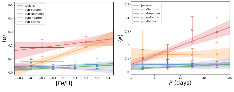
The central discovery is a size-dependent population eccentricity: small planets below roughly 3.5 Earth radii orbit on nearly circular paths with $\langle e \rangle \approx 0.05$, while larger planets have $\langle e \rangle \approx 0.20$. The transition appears in both single- and multi-transiting systems, with singles uniformly about 2.4 times more eccentric than multis. Because the same radius threshold also separates a common, metal-insensitive population of small planets from a rare, metal-rich population of large planets, the paper interprets the eccentricity jump as evidence that the two size groups formed through distinct dynamical pathways. The eccentricity distribution is self-similar in shape across size classes, peaking at $e = 0$ and declining monotonically, so the size effect is primarily a change in the spread of the distribution rather than its functional form.
Load-bearing premise
The load-bearing premise is that, after Gaussian-process detrending and transit-timing-variation correction, the measured transit durations are unbiased and the Gaia-based stellar densities are accurate, so any leftover duration anomaly is a real eccentricity signal rather than a size-dependent systematic error.
Editorial extensions
If this is right
- Large and small close-in planets must be explained by separate formation channels, one that preserves low eccentricities for sub-Neptune-sized bodies and one that excites eccentricities for larger planets.
- Models of planet occurrence must reproduce a coordinated break at roughly 3.5 Earth radii in eccentricity, occurrence rate, and host-star metallicity simultaneously.
- If the radius-valley eccentricity excess is real, gap planets likely formed through collisions or atmospheric stripping, a prediction testable with radial-velocity follow-up or JWST secondary-eclipse measurements.
- Single- and multi-transiting planets share one parent population, with singles representing the high-eccentricity, high-inclination tail, which bears on explanations of the Kepler dichotomy.
- For planets above 4 Earth radii, the positive eccentricity-metallicity and eccentricity-period correlations constrain when and how giant planet eccentricities are excited relative to disk dispersal.
Reading between the lines
- A natural extension is to test whether the 3.5 Earth-radius threshold shifts with stellar mass or orbital period, which would sharpen the formation-channel interpretation by separating intrinsic size effects from environmental ones.
- The same hierarchical photoeccentric machinery could be applied to TESS light curves, where shorter baselines and higher noise may require combining many systems to recover the same size-eccentricity signal.
- The paper's eccentricity-dilution argument implies that any small planet found with a confidently high eccentricity may be a marker for an unseen outer giant companion, a prediction that radial-velocity surveys could directly test.
- If the radius-valley eccentricity peak is confirmed, it would motivate targeted searches for collision remnants or stripped cores in that radius range using atmospheric and density measurements.
Editorial analysis
A structured set of objections, weighed in public.
Referee Report
Summary. This paper measures eccentricities for 1646 Kepler planets with periods 1–100 days and radii 0.5–16 R⊕, using the photoeccentric effect: transit durations from the ALDERAAN pipeline are compared to duration predictions from Gaia stellar densities via importance sampling, producing per-planet posterior samples in (e, ω). The authors then infer population eccentricity distributions with an approximate hierarchical Bayesian model using a non-parametric regularized histogram, later compressed into a two-parameter empirical template. The central claim is that mean population eccentricity rises from ⟨e⟩ = 0.05 ± 0.01 for planets smaller than about 3.5 R⊕ to ⟨e⟩ = 0.20 ± 0.03 for larger planets, and that this transition aligns with breaks in occurrence rate and host-star metallicity, implying distinct formation channels. Additional findings include a tentative (2.1σ) elevation of eccentricity for planets in the radius valley, and a single-to-multi eccentricity ratio of about 2.5 with similar ⟨e⟩–R_p curves for both populations.
Significance. If the size–eccentricity step is real, it is an important demographic signature that connects planet occurrence, composition, and dynamical history, and it sharpens the evidence for distinct formation channels around 3.5 R⊕. The paper's strengths are substantial: the analysis pipeline is open source; the authors run a large injection/recovery campaign; they check robustness across distributional choices (empirical, beta, half-Gaussian), binning schemes, selection cuts, and detection-bias corrections; they forward-model duration ratios; and they honestly report the weak 2.1σ radius-valley signal. The per-planet eccentricity constraints are weak (σ(e) ≈ 0.3), so the population claims rest on the ensemble analysis being unbiased as a function of planet radius. The main weakness is that the injection/recovery tests validate recovery of a step-like ground truth but do not test the null hypothesis of a size-independent eccentricity distribution; this missing test is directly relevant to the central claim.
major comments (2)
- [SI, Injection-and-recovery tests (Table 4, Figs. 15–20)] The validation simulations inject a step-like ground truth: small planets (Rp < 4 R⊕) drawn from a half-normal with σ = 0.03 (⟨e⟩ ≈ 0.023) and large planets drawn from a beta distribution with mean ≈ 0.23. The authors then show that the recovered ⟨e⟩ values are consistent with these injected values. This demonstrates that the pipeline can recover an injected step, but it does not test whether the pipeline could create a spurious step from a population whose eccentricity distribution is the same at all sizes. Because individual eccentricity posteriors have σ(e) ≈ 0.3, the reported rise from 0.05 to 0.20 is an ensemble-level statement; a size-dependent bias in measured T14 from, e.g., unaccounted TTV smearing, long-cadence smearing, or GP detrending could in principle produce the observed trend even if the intrinsic population is flat in planet size. The authors should inject a population with a single global f(e) (or size-independent template parameters) for all radii and show that the recovered ⟨e⟩–R_p relation is flat; analogous tests with a mild intrinsic slope would also constrain the pipeline response. This null test is the most important missing validation for the central claim.
- [Methods, Eq. (5); SI, Eq. (22)] The detection-bias correction in the hierarchical likelihood uses only the geometric transit probability, (1−e²)/(1+e sinω). However, Kepler's detection probability also depends on transit duration and depth, which are correlated with e and ω through the same photoeccentric relation. The injection/recovery tests do not simulate the full planet detection process: they inject synthetic transits into existing Kepler light curves and then fit them, so the recovered posteriors are conditioned on the transit being present and fitted, not on the original detection selection. The claim that Eq. (5) yields the intrinsic (rather than observed) eccentricity distribution is therefore not fully validated by the presented tests. This could affect the absolute scale of ⟨e⟩, and possibly the size-dependent trend if duration- and depth-dependent detectability vary with planet radius. I ask the authors to either add a duration-dependent detection term to Eq. (5) or demonstrate through a forward-modeled survey simulation (including the detection step) that the geometric correction alone is sufficient for the claimed precision.
minor comments (8)
- [Methods, first paragraph] The sentence "We first select a sample of 1209 single Sun-like stars hosing 1646 planets" contains a typo: "hosing" should be "hosting".
- [Introduction, paragraph 2] The phrase "has be remarkably successful at at explaining" contains duplicated words; please correct to "has been remarkably successful at explaining".
- [Conclusions, item 3] The phrase "Planets in the the radius valley" has a duplicated "the".
- [SI, Fig. 11 caption] The caption reads "for each of our five plannet size classes"; "plannet" should be "planet".
- [Abstract] The clause "a narrow band of low occurrence rate density which separates rocky ``super-Earths'' (1.0–1.5 Earth-radii) from gas-rich ``sub-Neptunes'' (2.0–3.0 Earth-radii" is missing a closing parenthesis after "Earth-radii".
- [SI, after Eq. (26)] The regularization term added to the log-likelihood, ln L = −(ν−h)², is ad hoc and not derived from the data; please justify its form and strength, or show that results are unchanged when this term is omitted (Figure 14 partially addresses this via alternative parametric models, but not for the template fit itself).
- [Methods, Table 1] The paper does not report the number of planets per size bin; given that the largest bins (R0 ≈ 14.6 R⊕) contain very few planets, the sigmoid fit parameters and their uncertainties would be more interpretable with effective sample sizes listed.
- [SI, Estimating the significance of the eccentricity peak in the radius valley] The combination of tail probabilities P(A_singles ≤ 0) and P(A_multis ≤ 0) treats the two measurements as independent, but they share the same empirical template and are drawn from the same parent population according to the paper's own conclusion; please discuss the sensitivity of the 2.1σ figure to this independence assumption.
Circularity Check
No significant circularity: the eccentricity measurements are inferred from external Kepler and Gaia data, and the size-eccentricity trend is not equivalent to any fitted input.
full rationale
The paper's central claim, that mean eccentricity rises from about 0.05 for small planets to about 0.20 for planets larger than roughly 3.5 Earth-radii, is derived from photoeccentric inversion of transit durations against Gaia-based stellar densities. The inference chain is self-contained: transit shapes are fit to Kepler photometry, eccentricity posteriors are obtained by importance sampling that compares the implied stellar density to the Gaia prior, and the hierarchical model fits population-level eccentricity distributions to those posteriors. The method relies on the authors' prior papers (refs 40 and 44), but that reliance is methodological rather than circular: the cited importance-sampling equivalence is a stated mathematical procedure, and the present paper validates the same pipeline with injection-and-recovery tests against external synthetic data. Those injections do simulate a step-like eccentricity ground truth, so they do not by themselves rule out a flat-truth systematic, but that is a validation limitation, not a circular reduction. The alignment with occurrence-rate and metallicity breaks is supported by independent catalog results (refs 57-59), and the radius-valley peak is tested with null injections that depopulate the gap. No equation in the paper reduces the size-eccentricity trend to a fitted parameter or to a self-referential definition.
Assumptions & free parameters
free parameters (6)
- Template tail weight nu per size class =
Jovians 0.68+0.31/-0.14; sub-Saturns 0.80+0.25/-0.16; sub-Neptunes 1.01+0.09/-0.06; super-Earths 1.60+0.34/-0.25…
- Template width scale h =
Jovians 0.55+0.27/-0.21; sub-Saturns 0.60+0.29/-0.20; sub-Neptunes 1.21+0.29/-0.23; super-Earths 1.02+0.28/-0.21…
- Sigmoid transition radius x_t =
Rp = 3.3 +/- 0.4 R_Earth (singles), 4.2 +/- 0.9 R_Earth (multis)
- Gaussian peak amplitude A in radius valley =
A > 0 in 73% (singles) and 89% (multis) of posterior samples
- GP smoothness hyperparameters ln(s), ln(l) =
ln(s) ~ N(3,1), ln(l) ~ N(0,1) hyperpriors
- Outlier correction epsilon =
1e-6
assumptions (6)
- standard math The transit duration formula T14 (Eq. 15) accurately describes the relation between observed duration and P, Rp/R*, b, e, omega, and rho*.
- domain assumption Gaia-derived stellar densities rho* are accurate to their quoted uncertainties and serve as the external calibration for eccentricity.
- domain assumption A uniform interim prior on e and omega (p0(e)=1) during importance sampling is appropriate.
- ad hoc to paper All planet size classes share the same functional form of f(e) up to the scaling parameters nu and h (Eq. 6).
- standard math The geometric transit probability p = (1 + e sin(omega)) / (1 - e^2) fully corrects the sample selection bias for eccentric orbits.
- ad hoc to paper The GP smoothness prior and the manual monotonicity enforcement on the histogram do not distort the inferred distribution shape.
invented entities (1)
-
Radius-valley 'gap planets' population
independent evidence
Cite this review
Pith. "Pith review of Planets larger than Neptune have elevated eccentricities." pith.science (2026). https://pith.science/paper/2IUFU2AY
@misc{pith2026250707840,
  author       = {Pith},
  title        = {Pith review of: Planets larger than Neptune have elevated eccentricities},
  year         = {2026},
  howpublished = {\url{https://pith.science/paper/2IUFU2AY}},
  note         = {Machine review of arXiv:2507.07840}
}
abstract
NASA's Kepler mission identified over 4000 extrasolar planets that transit (cross in front of) their host stars. This sample has revealed detailed features in the demographics of planet sizes and orbital spacings. However, knowledge of their orbital shapes - a key tracer of planetary formation and evolution - remains far more limited. We present measurements of eccentricities for 1646 Kepler planets, 92% of which are smaller than Neptune. For all planet sizes, the eccentricity distribution peaks at e=0 and falls monotonically toward zero at e=1. As planet size increases, mean population eccentricity rises from $\langle e \rangle = 0.05 \pm 0.01$ for small planets to $\langle e \rangle = 0.20 \pm 0.03$ for planets larger than $\sim$ 3.5 Earth-radii. The overall planet occurrence rate and planet-metallicity correlation also change abruptly at this size. Taken together, these patterns indicate distinct formation channels for planets above and below $\sim$ 3.5 Earth-radii. We also find size dependent associations between eccentricity, host star metallicity, and orbital period. While smaller planets generally have low eccentricities, there are hints of a noteworthy exception: eccentricities are slightly elevated in the ``radius valley,'' a narrow band of low occurrence rate density which separates rocky ``super-Earths'' (1.0-1.5 Earth-radii) from gas-rich ``sub-Neptunes'' (2.0-3.0 Earth-radii. We detect this feature at $2.1\sigma$ significance. Planets in single- and multi-transiting systems exhibit the same size-eccentricity relationship, suggesting they are drawn from the same parent population.
Figures


Figures from the paper (14 more)



Forward citations
Cited by 2 Pith papers
-
Dynamically Selected Mass-Radius Relationship for Low Mass Exoplanets
Planets inferred to have suffered giant collisions are more massive than pristine ones but retain comparable hydrogen envelope fractions, implying collisions occurred before disk gas dispersal.
-
Understanding eccentric temperate giants: an in-depth study of the architecture and stellar obliquity of the TOI-2134 system
Updated analysis of TOI-2134 with new TESS sectors and spectra confirms an inner mini-Neptune and outer eccentric sub-Saturn, measures their masses and radii, and reports a 59 degree obliquity for the outer planet via...
Reference graph
Works this paper leans on
-
[1]
PS Laplace, Exposition Du Système Du Monde . (1796)
-
[2]
Nature 435, 459–461 (2005)
K Tsiganis, R Gomes, A Morbidelli, HF Levison, Origin of the orbital architecture of the giant planets of the Solar System. Nature 435, 459–461 (2005)
2005
-
[3]
EA Petigura, AW Howard, GW Marcy, Prevalence of Earth-size planets orbiting Sun-like stars. Proc. Natl. Acad. Sci . 110, 19273–19278 (2013)
2013
-
[4]
ApJS 201, 15 (2012)
AW Howard, et al., Planet Occurrence within 0.25 AU of Solar-type Stars from Kepler. ApJS 201, 15 (2012)
2012
-
[5]
BJ Fulton, et al., The California-Kepler Survey. III. A Gap in the Radius Distribution of Small Planets. AJ 154, 109 (2017)
2017
-
[6]
MNRAS 392, 641–654 (2009)
SJ O’Toole, et al., Selection functions in doppler planet searches. MNRAS 392, 641–654 (2009)
2009
-
[7]
Science 274, 954–956 (1996)
FA Rasio, EB Ford, Dynamical instabilities and the formation of extrasolar planetary systems. Science 274, 954–956 (1996)
1996
-
[8]
ApJ 678, 1396–1406 (2008)
B Jackson, R Greenberg, R Barnes, Tidal Evolution of Close-in Extrasolar Planets. ApJ 678, 1396–1406 (2008)
2008
Show all 98 references
-
[9]
ARAA 56, 175–221 (2018)
RI Dawson, JA Johnson, Origins of Hot Jupiters. ARAA 56, 175–221 (2018)
2018
-
[10]
MNRAS 434, L51–L55 (2013)
DM Kipping, Parametrizing the exoplanet eccentricity distribution with the beta distribution. MNRAS 434, L51–L55 (2013)
2013
-
[11]
AJ 157, 61 (2019)
V Van Eylen, et al., The Orbital Eccentricity of Small Planet Systems. AJ 157, 61 (2019)
2019
-
[12]
DC Fabrycky, et al., Architecture of Kepler’s Multi-transiting Systems. II. New Investigations with Twice as Many Candidates. ApJ 790, 146 (2014)
2014
-
[13]
JW Xie, et al., Exoplanet orbital eccentricities derived from LAMOST -Kepler analysis.Proc. Natl. Acad. Sci . 113, 11431–11435 (2016)
2016
-
[14]
SM Mills, et al., The California-Kepler Survey. VIII. Eccentricities of Kepler Planets and Tentative Evidence of a High-metallicity Preference for Small Eccentric Planets. AJ 157, 198 (2019)
2019
-
[15]
ApJ 808, 126 (2015)
V Van Eylen, S Albrecht, Eccentricity from Transit Photometry: Small Planets in Kepler Multi-planet Systems Have Low Eccentricities. ApJ 808, 126 (2015)
2015
-
[16]
S Sagear, S Ballard, The orbital eccentricity distribution of planets orbiting M dwarfs. Proc. Natl. Acad. Sci . 120, e2217398120 (2023)
2023
-
[17]
Icarus 124, 62–85 (1996)
JB Pollack, et al., Formation of the Giant Planets by Concurrent Accretion of Solids and Gas. Icarus 124, 62–85 (1996)
1996
-
[18]
ApJ 686, 621–636 (2008)
EB Ford, FA Rasio, Origins of Eccentric Extrasolar Planets: Testing the Planet-Planet Scatter- ing Model. ApJ 686, 621–636 (2008)
2008
-
[19]
ApJ 669, 1298–1315 (2007)
D Fabrycky, S Tremaine, Shrinking Binary and Planetary Orbits by Kozai Cycles with Tidal Friction. ApJ 669, 1298–1315 (2007)
2007
-
[20]
MNRAS 501, 1621–1632 (2021)
J Li, D Lai, KR Anderson, B Pu, Giant planet scatterings and collisions: hydrodynamics, merger-ejection branching ratio, and properties of the remnants. MNRAS 501, 1621–1632 (2021)
2021
-
[21]
ApJ 585, 1024–1037 (2003)
P Goldreich, R Sari, Eccentricity Evolution for Planets in Gaseous Disks. ApJ 585, 1024–1037 (2003)
2003
-
[22]
SE Thompson, et al., Planetary Candidates Observed by Kepler. VIII. A Fully Automated Catalog with Measured Completeness and Reliability Based on Data Release 25. ApJS 235, 38 (2018)
2018
-
[23]
JL Christiansen, et al., Measuring Transit Signal Recovery in the Kepler Pipeline. IV. Com- pleteness of the DR25 Planet Candidate Catalog. AJ 160, 159 (2020)
2020
-
[24]
AJ 161, 36 (2021)
S Bryson, et al., The Occurrence of Rocky Habitable-zone Planets around Solar-like Stars from Kepler Data. AJ 161, 36 (2021)
2021
-
[25]
ApJ 866, 99 (2018)
TA Berger, D Huber, E Gaidos, JL van Saders, Revised Radii of Kepler Stars and Planets Using Gaia Data Release 2. ApJ 866, 99 (2018)
2018
-
[26]
TA Berger, et al., The Gaia-Kepler Stellar Properties Catalog. I. Homogeneous Fundamental Properties for 186,301 Kepler Stars. AJ 159, 280 (2020)
2020
-
[27]
E Furlan, et al., The Kepler Follow-up Observation Program. I. A Catalog of Companions to Kepler Stars from High-Resolution Imaging. AJ 153, 71 (2017)
2017
-
[28]
AJ 162, 128 (2021)
ML Wood, AW Mann, AL Kraus, Characterizing Undetected Stellar Companions with Combined Data Sets. AJ 162, 128 (2021)
2021
-
[29]
EA Petigura, et al., The California-Kepler Survey. X. The Radius Gap as a Function of Stellar Mass, Metallicity, and Age. AJ 163, 179 (2022)
2022
-
[30]
P ASP124, 985 (2012)
MC Stumpe, et al., Kepler Presearch Data Conditioning I—Architecture and Algorithms for Error Correction in Kepler Light Curves. P ASP124, 985 (2012)
2012
-
[31]
T Holczer, et al., Transit Timing Observations from Kepler. IX. Catalog of the Full Long-cadence Data Set. ApJS 225, 9 (2016)
2016
-
[32]
MNRAS 440, 2164– 2184 (2014)
DM Kipping, Characterizing distant worlds with asterodensity profiling. MNRAS 440, 2164– 2184 (2014)
2014
-
[33]
Summary of the contents and survey proper- ties
Gaia Collaboration, et al., Gaia Data Release 2. Summary of the contents and survey proper- ties. AA 616, A1 (2018)
2018
-
[34]
A@AND@A 553, A6 (2013)
TO Husser, et al., Astrophysics A new extensive library of PHOENIX stellar atmospheres. A@AND@A 553, A6 (2013)
2013
-
[35]
MNRAS 453, 3821–3826 (2015)
H Parviainen, S Aigrain, ldtk: Limb Darkening Toolkit. MNRAS 453, 3821–3826 (2015)
2015
-
[36]
IEEE T ransactions on Autom
H Akaike, A new look at the statistical model identification. IEEE T ransactions on Autom. Control. 19, 716–723 (1974)
1974
-
[37]
MNRAS 435, 2152–2160 (2013)
DM Kipping, Efficient, uninformative sampling of limb darkening coefficients for two-parameter laws. MNRAS 435, 2152–2160 (2013)
2013
-
[38]
AJ 163, 111 (2022)
GJ Gilbert, Accurate Modeling of Grazing Transits Using Umbrella Sampling. AJ 163, 111 (2022)
2022
-
[39]
AJ 160, 89 (2020)
EA Petigura, Two Views of the Radius Gap and the Role of Light Curve Fitting. AJ 160, 89 (2020)
2020
-
[40]
AJ 164, 92 (2022)
GJ Gilbert, MG MacDougall, EA Petigura, Implicit Biases in Transit Models Using Stellar Pseudo Density. AJ 164, 92 (2022)
2022
-
[41]
R Fischer, R Preuss, UV Toussaint
J Skilling, Nested Sampling in Bayesian Inference and Maximum Entropy Methods in Science and Engineering: 24th International Workshop on Bayesian Inference and Maximum Entropy Methods in Science and Engineering , American Institute of Physics Conference Series, eds. R Fischer,...
2004
-
[42]
E Higson, W Handley, M Hobson, A Lasenby, Dynamic nested sampling: an improved algorithm for parameter estimation and evidence calculation. Stat. Comput . 29, 891–913 (2019)
2019
-
[43]
MNRAS 493, 3132–3158 (2020)
JS Speagle, DYNESTY: a dynamic nested sampling package for estimating Bayesian posteri- ors and evidences. MNRAS 493, 3132–3158 (2020)
2020
-
[44]
AJ 166, 61 (2023)
MG MacDougall, GJ Gilbert, EA Petigura, Accurate and Efficient Photoeccentric Transit Modeling. AJ 166, 61 (2023)
2023
-
[45]
ApJ 678, 1407–1418 (2008)
EB Ford, SN Quinn, D Veras, Characterizing the Orbital Eccentricities of Transiting Extrasolar Planets with Photometric Observations. ApJ 678, 1407–1418 (2008)
2008
-
[46]
RI Dawson, JA Johnson, The Photoeccentric Effect and Proto-hot Jupiters. I. Measuring Photometric Eccentricities of Individual Transiting Planets. ApJ 756, 122 (2012)
2012
-
[47]
S Seager
JN Winn, Exoplanet Transits and Occultations in Exoplanets, ed. S Seager. pp. 55–77 (2010)
2010
-
[48]
ApJ 725, 2166–2175 (2010)
DW Hogg, AD Myers, J Bovy, Inferring the Eccentricity Distribution. ApJ 725, 2166–2175 (2010)
2010
-
[49]
AJ 159, 63 (2020)
BP Bowler, SC Blunt, EL Nielsen, Population-level Eccentricity Distributions of Imaged Exo- planets and Brown Dwarf Companions: Dynamical Evidence for Distinct Formation Channels. AJ 159, 63 (2020)
2020
-
[50]
P ASP119, 986–993 (2007)
JW Barnes, Effects of Orbital Eccentricity on Extrasolar Planet Transit Detectability and Light Curves. P ASP119, 986–993 (2007)
2007
-
[51]
ApJ 679, 1566–1573 (2008)
CJ Burke, Impact of Orbital Eccentricity on the Detection of Transiting Extrasolar Planets. ApJ 679, 1566–1573 (2008)
2008
-
[52]
MNRAS 444, 2263–2269 (2014)
DM Kipping, Bayesian priors for the eccentricity of transiting planets. MNRAS 444, 2263–2269 (2014)
2014
-
[53]
ApJ 795, 64 (2014)
D Foreman-Mackey, DW Hogg, TD Morton, Exoplanet Population Inference and the Abundance of Earth Analogs from Noisy, Incomplete Catalogs. ApJ 795, 64 (2014)
2014
-
[54]
MNRAS 510, 5623–5638 (2022)
K Masuda, EA Petigura, OJ Hall, Inferring the rotation period distribution of stars from their projected rotation velocities and radii: Application to late-F/early-G Kepler stars. MNRAS 510, 5623–5638 (2022)
2022
-
[55]
MA Newton, AE Raftery, Approximate Bayesian Inference with the Weighted Likelihood Bootstrap. J. R. Stat. 56, 3–26 (2018)
2018
-
[56]
MNRAS 519, 4056–4073 (2023)
CSK Ho, V Van Eylen, A deep radius valley revealed by Kepler short cadence observations. MNRAS 519, 4056–4073 (2023)
2023
-
[57]
BJ Fulton, EA Petigura, The California-Kepler Survey. VII. Precise Planet Radii Leveraging Gaia DR2 Reveal the Stellar Mass Dependence of the Planet Radius Gap. AJ 156, 264 (2018)
2018
-
[58]
Nature 486, 375–377 (2012)
LA Buchhave, et al., An abundance of small exoplanets around stars with a wide range of metallicities. Nature 486, 375–377 (2012)
2012
-
[59]
EA Petigura, et al., The California-Kepler Survey. IV. Metal-rich Stars Host a Greater Diversity of Planets. AJ 155, 89 (2018)
2018
-
[60]
ApJ 622, 1102–1117 (2005)
DA Fischer, J Valenti, The Planet-Metallicity Correlation. ApJ 622, 1102–1117 (2005)
2005
-
[61]
ApJ 860, 101 (2018)
W Zhu, C Petrovich, Y Wu, S Dong, J Xie, About 30% of Sun-like Stars Have Kepler-like Planetary Systems: A Study of Their Intrinsic Architecture. ApJ 860, 101 (2018)
2018
-
[62]
AJ 158, 109 (2019)
DC Hsu, EB Ford, D Ragozzine, K Ashby, Occurrence Rates of Planets Orbiting FGK Stars: Combining Kepler DR25, Gaia DR2, and Bayesian Inference. AJ 158, 109 (2019)
2019
-
[63]
ARAA 49, 67–117 (2011)
JP Williams, LA Cieza, Protoplanetary Disks and Their Evolution. ARAA 49, 67–117 (2011)
2011
-
[64]
arXiv e-prints p
Q Chance, S Ballard, Evidence that Planets in the Radius Gap Do Not Resemble Their Neighbors. arXiv e-prints p. arXiv:2410.02150 (2024)
2024 arXiv
-
[65]
AJ 168, 239 (2024)
F Dai, et al., The Prevalence of Resonance Among Y oung, Close-in Planets. AJ 168, 239 (2024)
2024
-
[66]
ApJ 847, 29 (2017)
JE Owen, Y Wu, The Evaporation Valley in the Kepler Planets. ApJ 847, 29 (2017)
2017
-
[67]
ApJ 792, 1 (2014)
ED Lopez, JJ Fortney, Understanding the Mass-Radius Relation for Sub-neptunes: Radius as a Proxy for Composition. ApJ 792, 1 (2014)
2014
-
[68]
ApJS 197, 8 (2011)
JJ Lissauer, et al., Architecture and Dynamics of Kepler’s Candidate Multiple Transiting Planet Systems. ApJS 197, 8 (2011)
2011
-
[69]
ApJ 816, 66 (2016)
S Ballard, JA Johnson, The Kepler Dichotomy among the M Dwarfs: Half of Systems Contain Five or More Coplanar Planets. ApJ 816, 66 (2016)
2016
-
[70]
MY He, EB Ford, D Ragozzine, D Carrera, Architectures of Exoplanetary Systems. III. Eccen- tricity and Mutual Inclination Distributions of AMD-stable Planetary Systems. AJ 160, 276 (2020)
2020
-
[71]
AJ 162, 166 (2021)
SC Millholland, et al., Evidence for a Nondichotomous Solution to the Kepler Dichotomy: Mutual Inclinations of Kepler Planetary Systems from Transit Duration Variations. AJ 162, 166 (2021)
2021
-
[72]
MNRAS 483, 4479–4494 (2019)
JK Zink, JL Christiansen, BMS Hansen, Accounting for incompleteness due to transit multiplic- ity in Kepler planet occurrence rates. MNRAS 483, 4479–4494 (2019)
2019
-
[74]
T Mazeh, et al., Transit Timing Observations from Kepler. VIII. Catalog of Transit Timing Measurements of the First Twelve Quarters. ApJS 208, 16 (2013)
2013
-
[75]
Econometrica 46, 1–19 (1978)
T Kloek, HK van Dijk, Bayesian estimates of equation system parameters: An application of integration by monte carlo. Econometrica 46, 1–19 (1978)
1978
-
[76]
(Taylor & Francis), (2013)
A Gelman, et al., Bayesian Data Analysis, Third Edition , Chapman & Hall/CRC Texts in Statistical Science. (Taylor & Francis), (2013)
2013
-
[77]
arXiv e-prints p
M Betancourt, A Conceptual Introduction to Hamiltonian Monte Carlo. arXiv e-prints p. arXiv:1701.02434 (2017)
2017 arXiv
-
[78]
JF Rowe, et al., Validation of Kepler’s Multiple Planet Candidates. III. Light Curve Analysis and Announcement of Hundreds of New Multi-planet Systems. ApJ 784, 45 (2014)
2014
-
[79]
JF Rowe, et al., Planetary Candidates Observed by Kepler. V. Planet Sample from Q1-Q12 (36 Months). ApJS 217, 16 (2015)
2015
-
[80]
PeerJ Comput
J Salvatier, TV Wiecki, C Fonnesbeck, Probabilistic programming in python using pymc3. PeerJ Comput. Sci. 2, e55 (2016)
2016
-
[81]
AJ 154, 220 (2017)
D Foreman-Mackey, E Agol, S Ambikasaran, R Angus, Fast and Scalable Gaussian Process Modeling with Applications to Astronomical Time Series. AJ 154, 220 (2017)
2017
-
[82]
arXiv e-prints p
MD Hoffman, A Gelman, The No-U-Turn Sampler: Adaptively Setting Path Lengths in Hamilto- nian Monte Carlo. arXiv e-prints p. arXiv:1111.4246 (2011)
2011 arXiv
-
[83]
R Neal, MCMC Using Hamiltonian Dynamics . pp. 113–162 (2011)
2011
-
[84]
A Gelman, DB Rubin, Inference from Iterative Simulation Using Multiple Sequences. Stat. Sci. 7, 457–472 (1992)
1992
-
[85]
The Annals Stat
G Schwarz, Estimating the Dimension of a Model. The Annals Stat . 6, 461 – 464 (1978)
1978
-
[86]
MNRAS 463, 1323–1331 (2016)
DM Kipping, E Sandford, Observational biases for transiting planets. MNRAS 463, 1323–1331 (2016)
2016
-
[87]
Giorn Dell’inst Ital Degli Att 4, 89–91 (1933)
K AN, Sulla determinazione empirica di una legge didistribuzione. Giorn Dell’inst Ital Degli Att 4, 89–91 (1933)
1933
-
[88]
Recueil Math
N Smirnov, Ob uklonenijah empiriceskoi krivoi raspredelenija. Recueil Math. (Matematiceskii Sbornik), NS 6, 3–26 (1939)
1939
-
[89]
TW Anderson, DA Darling, A test of goodness of fit. J. Am. Stat. Assoc . 49, 765–769 (1954)
1954
-
[90]
The Annals Math
S Kullback, RA Leibler, On Information and Sufficiency. The Annals Math. Stat . 22, 79 – 86 (1951)
1951
-
[91]
B Efron, Bootstrap Methods: Another Look at the Jackknife. Ann. Stat. 7, 1 – 26 (1979)
1979
-
[92]
AJ 158, 4 (2019)
KK O’Neil, et al., Improving Orbit Estimates for Incomplete Orbits with a New Approach to Priors: with Applications from Black Holes to Planets. AJ 158, 4 (2019)
2019
-
[93]
AJ 156, 123 (2018)
Astropy Collaboration, et al., The Astropy Project: Building an Open-science Project and Status of the v2.0 Core Package. AJ 156, 123 (2018)
2018
-
[94]
P ASP127, 1161 (2015)
L Kreidberg, batman: BAsic Transit Model cAlculatioN in Python. P ASP127, 1161 (2015)
2015
-
[95]
D Foreman-Mackey, et al., exoplanet: Gradient-based probabilistic inference for exoplanet data & other astronomical time series. The J. Open Source Softw . 6, 3285 (2021)
2021
-
[96]
Nature 585, 357–362 (2020)
CR Harris, et al., Array programming with NumPy. Nature 585, 357–362 (2020)
2020
-
[97]
S van der Walt, J Millman
W McKinney, Data structures for statistical computing in python in Proceedings of the 9th Python in Science Conference , eds. S van der Walt, J Millman. pp. 51 – 56 (2010)
2010
-
[98]
P Virtanen, et al., SciPy 1.0: Fundamental Algorithms for Scientific Computing in Python. Nat. Methods 17, 261–272 (2020)
2020
-
[99]
interim” prior one applied during model fitting (or in our case, during importance sampling) andf(e;α) is the informative “updated
R Luger, et al., starry: Analytic Occultation Light Curves. AJ 157, 64 (2019). Gilbert et al. PNAS | September 6, 2025 | vol. XXX | no. XX | 11 Supporting Information for Planets larger than Neptune have Elevated Eccentricities Gregory J. Gilbert, Erik A. Petigura, and Paige M...
2019 doi
Reviewed August 6, 2026 · model on record in the stance chip above.
Discussion (0). Continue with ORCID to comment.