REVIEW 4 major objections 5 minor 41 references
Energy Dissipation Rate Guided Adaptive Sampling for Physics-Informed Neural Networks: Resolving Surface-Bulk Dynamics in Allen-Cahn Systems
T0 review · 4 major / 5 minor · reviewed 2026-08-06 · deepseek-v4-flash
Pith's one-line read Sampling collocation points by local energy dissipation rate density, rather than by PDE residual, cuts the relative mean-square error of PINN solutions to the Allen-Cahn equation by up to a factor of six while using lower-order…
desk verdict A genuinely new PINN sampling idea with a strong 1D demo, but the algorithm as printed is internally inconsistent and not reproducible until fixed. read the letter →
The pith
A machine-rendered reading of the paper's core claim, the machinery that carries it, and where it could break.
The reading
What carries the argument
The load-bearing object is the local energy dissipation rate density $e_{edr}^f=\phi_t^2/M_b$ for the bulk and $e_{edr}^b=\phi_t^2/M_s$ for the boundary, used as an importance metric for resampling. The method computes it from the flux $\phi_t$ rather than from the chemical potential $\mu$, which requires higher-order derivatives, and it maintains domain coverage through a density-aware threshold that enforces a minimum number of points per subdomain while adding the highest-dissipation candidates. This machinery connects adaptive sampling to the Lyapunov structure of the free energy, concentrating training points where the solution's variance is large.
What would settle it
Run EDRAS on a thermodynamically consistent Allen-Cahn problem with a slowly moving flat interface where the local dissipation rate is low but the interface-position error is large; if EDRAS fails to concentrate points there and matches RAR's error level, the guiding-metric assumption would be contradicted.
Extended reading notes
Core claim
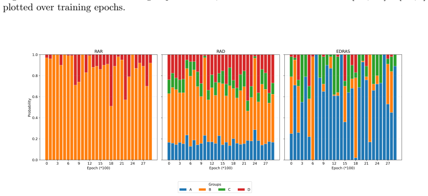
The paper's central discovery is that the local energy dissipation rate density, computed as $\phi_t^2/M_b$ in the bulk and $\phi_t^2/M_s$ on the boundary, is a more reliable sampling guide than the PDE residual for PINNs solving thermodynamically consistent Allen-Cahn systems. In a probabilistic analysis, residual-based refinement with a limited budget selects only points with large residuals (groups B and D) and never the small-residual, large-error points (group A); EDRAS samples from both critical groups and attains a higher probability of selecting high-error points than either RAR or RAD. The numerical experiments show that EDRAS reduces the relative MSE from $6.06\times10^{-4}$ to $1.08\times10^{-4}$ in the 1D periodic case, and that even mixing EDRAS with RAR markedly improves accuracy over RAR alone.
Load-bearing premise
The method works only if the places where the approximate neural-network solution dissipates energy fastest are also the places where its approximation error is largest; the paper demonstrates this correlation in one 1D example but does not prove it in general.
Editorial extensions
If this is right
- EDRAS can be attached to any PINN solver for a thermodynamically consistent model with a known free energy functional, without changing the network architecture or optimizer.
- For the Allen-Cahn equation, EDRAS alone outperforms residual-based adaptive refinement on MSE, MAE, and $L^\infty$ error, and combining it with RAR already gives most of the improvement.
- Because EDRAS avoids estimating the normalization $\int_\Omega R(y)\,dy$ needed by RAD and RAR-D, it is better suited to high-dimensional problems where that integral becomes intractable.
- In 2D disk and ellipse domains, higher surface mobility in dynamic boundary conditions accelerates boundary coarsening and slightly accelerates bulk energy decay, indicating surface mobility can act as a control parameter for bulk dynamics.
- The density threshold $d_f^{(0)}$ has a non-monotonic effect on accuracy: moderate increases reduce error, but too high a threshold degrades performance, so the method requires tuning this hyperparameter.
Reading between the lines
- An editorial extension is that the same dissipation-density heuristic should transfer to other gradient flows such as Cahn-Hilliard and phase-field crystal models, where $\phi_t^2/M$ is still the natural local dissipation indicator.
- If the dissipation-error correlation holds beyond Allen-Cahn, EDRAS could serve as a cheap a posteriori error estimator inside classical mesh adaptivity, not only inside neural-network training.
- A testable extension is to compare EDRAS with RAD on a two- or three-dimensional thermodynamically consistent problem to verify that the computational saving grows with dimension, as the paper argues from the cost of the normalization factor.
- A natural hybrid would weight dissipation density and residual together; the paper's group analysis suggests such a blend could hedge against regimes where a dynamically active region is already well approximated.
Editorial analysis
A structured set of objections, weighed in public.
Referee Report
Summary. The manuscript introduces EDRAS, an adaptive collocation-point sampling strategy for PINNs that uses the local energy dissipation rate density of a thermodynamically consistent model as the guide for adding and removing training points, instead of the PDE residual. The method is applied to the Allen-Cahn equation in 1D with periodic boundary conditions and in 2D disk/ellipse domains with Neumann or dynamic boundary conditions. The authors report up to a sixfold reduction in relative MSE compared with residual-based adaptive refinement (RAR) in the 1D benchmark, provide a probability-based argument for why RAR can miss low-residual/high-error regions, and draw qualitative conclusions about how surface mobility affects bulk dynamics. The 1D and 2D Neumann cases are validated against finite-difference reference solutions; the dynamic-boundary cases are not.
Significance. If the central claim is established, EDRAS would be a useful and computationally cheap alternative to residual-based adaptive sampling for dissipative PDEs, because it replaces higher-order residual derivatives with a first-order dissipation-rate density and requires no global density estimation. The 1D benchmark is clean and uses an external FDM reference, which avoids circularity, and the probability-based comparison in Figures 6-7 is a helpful conceptual explanation of a known limitation of RAR. However, the evidence for superiority over RAR is currently limited to one 1D problem, the printed algorithm is internally inconsistent in its definition of the sampling metric, and the physical insights from the dynamic-boundary cases are not independently validated. The method also has several under-specified hyperparameters. These issues are fixable, and the underlying idea is promising.
major comments (4)
- [Algorithm 1, steps 2-3 and 8; Eq. (3); Eq. (11); Section 2.2] The definition of the EDRAS metric in Algorithm 1 is inconsistent with the model's thermodynamics. Eq. (3) gives the bulk dissipation-rate integrand as -phi_t^2/M_b (and Eq. (11) as -phi_t^2/5), and Section 2.2 states that eedrdf is the absolute value of the energy dissipation-rate density, so eedrdf should be phi_t^2/M_b or at least |phi_t|/M_b. Algorithm 1 instead sets eedrdf = phi_t/M_b and uses this signed quantity in the thresholding (step 3) and in the top-m selection (step 8). Since phi_t changes sign during Allen-Cahn evolution, this is not a dissipation-rate density: regions with large negative phi_t are removed regardless of magnitude, while regions with small positive phi_t can be retained. The threshold eedrdf0 can itself become negative under this definition. The resampled point sets that produce the reported results in Table 1 and Figures 5 and 7 therefore depend on which of phi_t/M_b, |phi_t|/M_b, or phi_t^2/M_b was actually implemented. Please correct the algorithm to match the thermodynamics and state which quantity was used in each experiment; without this, the central numerical claim is not reproducible from the printed method.
- [Section 3.2, Table 2; Section 3.3; Abstract] The paper's headline claim is that EDRAS outperforms RAR, but the only head-to-head quantitative comparison is the 1D periodic problem in Table 1. In the 2D Neumann case, Section 3.2 says adaptive refinement was performed with EDRAS and RAR methods independently or in combination, yet Table 2 and Figure 8 report only EDRAS errors against the FDM reference; no RAR-only or combined 2D error metrics are shown. The 2D dynamic-boundary studies in Section 3.3 contain no reference solution and no RAR comparison. Consequently, the abstract's implication that EDRAS improves PINNs in arbitrary domains relative to RAR is supported only by a single 1D benchmark. Please add at least one 2D comparison, such as the disk with Neumann boundary conditions, under identical training settings, with error metrics for RAR, EDRAS, and EDRAS+RAR.
- [Section 3.3, Figures 10-13; Section 3.2] The physical conclusions about dynamic boundary conditions, e.g., that higher surface mobility accelerates boundary coarsening and slightly accelerates bulk energy decay, are drawn exclusively from PINN solutions with dynamic boundary conditions. No independent reference solution or error estimate is provided for these cases; the only external 2D validation is for the Neumann case (Table 2). Because EDRAS is a heuristic sampling strategy, the observed differences between Ms=10 and Ms=2 or 5 could lie within the approximation error of the PINN. Please validate at least one dynamic-boundary configuration against an FDM or other grid-converged reference, or explicitly rephrase these conclusions as qualitative observations that are not quantitatively established.
- [Algorithm 1; Section 2.2; Section 3.2, Table 3] The algorithm depends on the number of subdomains N, the density thresholds d_f^(0) and d_b^(0), and the 1/3 factor in the dissipation threshold. The manuscript never states the value of N used in the experiments, and the description of d_f^(0) as being determined from the total number of points in a uniform grid is not a precise recipe in a mesh-free PINN setting. The 1/3 factor is introduced without justification or sensitivity analysis; Table 3 varies d_f^(0) but not the 1/3 factor or N. These choices directly affect which points are added and removed, so the method as printed is not fully reproducible. Please provide the exact parameter values used in each numerical experiment and include a brief sensitivity discussion for the 1/3 factor.
minor comments (5)
- [Figure 7 caption, Section 3.1] The caption states that 'EDRAS focuses exclusively on the error', but EDRAS selects points using the energy dissipation-rate density, which the paper argues is a proxy for error; the wording should be corrected to avoid implying that the error itself is used in the sampling criterion.
- [Section 3.1, probability discussion] The statement pRAR(B\cup D)=1 is a conditional conclusion that holds only when m is small enough that every selected top-m residual exceeds the threshold R0; the manuscript should state this condition explicitly rather than presenting it as unconditional.
- [Eq. (3) and Eq. (18)] The dissipation-rate density is written with a leading minus inside the integrand; writing E'(t) = -\int_\Omega phi_t^2/M_b dx - \int_{\partial\Omega} phi_t^2/M_s dS would avoid any ambiguity about the sign of phi_t^2.
- [Algorithm 1, step 3] The phrase 'density of bulk energy dissipation rate density' is redundant; consider using 'bulk energy dissipation-rate density' throughout the algorithm.
- [Data Availability] The statement that no data were used is surprising given the extensive numerical experiments; if the simulations are reproducible from the described code, the authors should state that simulation data are available on request or deposit the code.
Circularity Check
No load-bearing circularity: EDRAS accuracy is benchmarked against an external FDM reference; self-citations are non-load-bearing; Algorithm 1's eedrdf = phi_t/M_b is inconsistent with the dissipation density phi_t^2/M_b of Eq. (3), a reproducibility flaw rather than a circular step.
full rationale
The paper's central numerical claims — the up-to-sixfold relative-MSE reduction of EDRAS over RAR (Table 1) and the higher sampling probability that EDRAS lands in the high-error groups A union B (Figure 7) — are evaluated against an external finite-difference reference, not against the method's own training data: the paper states that the reference solution is computed using the finite difference method (Section 3.1), and the 2D validation similarly benchmarks against a reference solution obtained using finite difference methods [39]. The dissipation-to-error correspondence that motivates EDRAS is presented as an empirically tested heuristic (Figure 2; the group-probability experiment with error threshold e0 = 0.001 and residual threshold R0 equal to the mean residual), not derived as an identity, so sampling by dissipation density is not equivalent by construction to reducing the FDM-based error. The self-citations are real but not load-bearing: the governing system (2) and the dissipation identities (3), (11), (18), (20) are re-derived in-paper by direct calculation, so the thermodynamic-consistency premise does not rest solely on [3] (first author's dissertation) or [16,17] (Jing and Wang, with the corresponding author); and the cited well-posedness results are external ([2,7,8,9,29,30,37]). Reference [39] is a submitted same-group paper, but finite differences are an independent discretization paradigm, externally falsifiable, hence genuine evidence under the stated rules. Two caveats, neither an input-output reduction: (i) Algorithm 1, step 3, defines the sampling metric as eedrdf = phi_t/M_b, whereas the text defines it as the absolute value of the energy dissipation rate density in the bulk, which Eq. (3) gives as phi_t^2/M_b; because phi_t changes sign under Allen-Cahn dynamics, the printed algorithm is ambiguous (phi_t/M_b vs |phi_t|/M_b vs phi_t^2/M_b), and the choice changes which points are pruned and added, clouding reproducibility of Table 1 and Figures 5 and 7 — a correctness flaw, not circularity. (ii) The dynamic-boundary-condition insights (Section 3.3, Figures 10-13) are read off PINN+EDRAS solutions without an independent dynamic-BC solver, leaving them unvalidated rather than self-referential. No derivation step collapses into its own input, so the circularity score is minimal.
Assumptions & free parameters
free parameters (4)
- Dissipation threshold fraction 1/3 =
1/3
- Density threshold d0_f (and d0_b) =
100-300 in experiments (Table 3)
- Number of subdomains N for density detection =
not specified
- Time-marching segment breakpoints =
T1=0.01, T2-T6 in [0.2,1.0] in 1D; uniform dt=0.2 with initial 0.01 in 2D
assumptions (5)
- domain assumption Generalized Onsager principle yields thermodynamically consistent Allen-Cahn equations with dynamic boundary conditions (system 2).
- ad hoc to paper The local energy dissipation rate density of the approximate PINN solution is a reliable proxy for the local approximation error.
- domain assumption The finite difference reference solutions are accurate enough to serve as ground truth.
- standard math The frequency principle / spectral bias of neural networks describes the training difficulty (low to high frequencies).
- standard math The Allen-Cahn equation with double-well potential is thermodynamically consistent and has an energy dissipation inequality (equation 3).
Cite this review
Pith. "Pith review of Energy Dissipation Rate Guided Adaptive Sampling for Physics-Informed Neural Networks: Resolving Surface-Bulk Dynamics in Allen-Cahn Systems." pith.science (2026). https://pith.science/paper/Y3MU7BH6
@misc{pith2026250709757,
  author       = {Pith},
  title        = {Pith review of: Energy Dissipation Rate Guided Adaptive Sampling for Physics-Informed Neural Networks: Resolving Surface-Bulk Dynamics in Allen-Cahn Systems},
  year         = {2026},
  howpublished = {\url{https://pith.science/paper/Y3MU7BH6}},
  note         = {Machine review of arXiv:2507.09757}
}
read the original abstract
We introduce the Energy Dissipation Rate guided Adaptive Sampling (EDRAS) strategy, a novel method that substantially enhances the performance of Physics-Informed Neural Networks (PINNs) in solving thermodynamically consistent partial differential equations (PDEs) over arbitrary domains. EDRAS leverages the local energy dissipation rate density as a guiding metric to identify and adaptively re-sample critical collocation points from both the interior and boundary of the computational domain. This dynamical sampling approach improves the accuracy of residual-based PINNs by aligning the training process with the underlying physical structure of the system. In this study, we demonstrate the effectiveness of EDRAS using the Allen-Cahn phase field model in irregular geometries, achieving up to a sixfold reduction in the relative mean square error compared to traditional residual-based adaptive refinement (RAR) methods. Moreover, we compare EDRAS with other residual-based adaptive sampling approaches and show that EDRAS is not only computationally more efficient but also more likely to identify high-impact collocation points. Through numerical solutions of the Allen-Cahn equation with both static (Neumann) and dynamic boundary conditions in 2D disk- and ellipse-shaped domains solved using PINN coupled with EDRAS, we gain significant insights into how dynamic boundary conditions influence bulk phase evolution and thermodynamic behavior. The proposed approach offers an effective, physically informed enhancement to PINN frameworks for solving thermodynamically consistent models, making PINN a robust and versatile computational tool for investigating complex thermodynamic processes in arbitrary geometries.
Figures


Figures from the paper (19 more)



Reference graph
Works this paper leans on
-
[1]
Learn Singularly Perturbed Solutions via Homotopy Dynamics
Chuqi Chen, Yahong Yang, Yang Xiang, and Wenrui Hao. Learn sharp interface solution by homotopy dynamics.arXiv preprint arXiv:2502.00488, 2025
work page Pith review arXiv 2025
-
[2]
Univ., Fachbereich Mathematik und Informatik, 2004
Ralph Chill, Eva Fašangová, and Jan Prüss.Convergence to Steady States of Solutions of the Cahn-Hilliard Equation with Dynamic Boundary Conditions. Univ., Fachbereich Mathematik und Informatik, 2004
work page 2004
-
[3]
L. Chunyan.Deep Learning for Studying Materials Stability and Solving Thermodynamically Consistent PDEs with Dynamic Boundary Conditions in Arbitrary Domains. Doctoral disser- tation, 2023
work page 2023
-
[4]
ArkaDaw, JieBu, SifanWang, ParisPerdikaris, andAnujKarpatne. Rethinkingtheimportance of sampling in physics-informed neural networks.arXiv preprint arXiv:2207.02338, 2022
arXiv 2022
-
[5]
Luis Espath. A continuum framework for phase field with bulk-surface dynamics.Partial Differential Equations and Applications, 4(1):1, 2023. 25
work page 2023
-
[6]
Henri Faure and Christiane Lemieux. Generalized halton sequences in 2008: A comparative study.ACM Transactions on Modeling and Computer Simulation (TOMACS),19(4):1–31, 2009
work page 2008
-
[7]
Ciprian G Gal. A cahn–hilliard model in bounded domains with permeable walls.Mathematical methods in the applied sciences, 29(17):2009–2036, 2006
work page 2009
-
[8]
The non-isothermal allen-cahn equation with dynamic boundary conditions.Discrete Contin
Ciprian G Gal, Maurizio Grasselli, et al. The non-isothermal allen-cahn equation with dynamic boundary conditions.Discrete Contin. Dyn. Syst, 22(4):1009–1040, 2008
work page 2008
Show all 41 references
-
[9]
On the cahn–hilliard equation with irregular potentials and dynamic boundary conditions.Commun
Gianni Gilardi, Alain Miranville, Giulio Schimperna, et al. On the cahn–hilliard equation with irregular potentials and dynamic boundary conditions.Commun. Pure Appl. Anal, 8(3):881– 912, 2009
2009
-
[10]
Tcas-pinn: Physics-informed neural networks with a novel temporal causality-based adaptive sampling method.Chinese Physics B, 33(5):050701, 2024
Jia Guo, Haifeng Wang, Shilin Gu, and Chenping Hou. Tcas-pinn: Physics-informed neural networks with a novel temporal causality-based adaptive sampling method.Chinese Physics B, 33(5):050701, 2024
2024
-
[11]
On the efficiency of certain quasi-random sequences of points in evaluating multi-dimensional integrals.Numerische Mathematik, 2:84–90, 1960
John H Halton. On the efficiency of certain quasi-random sequences of points in evaluating multi-dimensional integrals.Numerische Mathematik, 2:84–90, 1960
1960
-
[12]
Springer Science & Business Media, 2013
John Hammersley.Monte carlo methods. Springer Science & Business Media, 2013
2013
-
[13]
Monte carlo methods for solving multivariable problems.Annals of the New York Academy of Sciences, 86(3):844–874, 1960
John M Hammersley. Monte carlo methods for solving multivariable problems.Annals of the New York Academy of Sciences, 86(3):844–874, 1960
1960
-
[14]
Residual-quantile adjustment for adaptive training of physics-informed neural network
Jiayue Han, Zhiqiang Cai, Zhiyou Wu, and Xiang Zhou. Residual-quantile adjustment for adaptive training of physics-informed neural network. In2022 IEEE International Conference on Big Data (Big Data), pages 921–930. IEEE, 2022
2022
-
[15]
Multiscale neural networks for approximating green’s functions.arXiv preprint arXiv:2410.18439, 2024
Wenrui Hao, Rui Peng Li, Yuanzhe Xi, Tianshi Xu, and Yahong Yang. Multiscale neural networks for approximating green’s functions.arXiv preprint arXiv:2410.18439, 2024
2024
-
[16]
Thermodynamically consistent models for coupled bulk and surface dynamics.Entropy, 24(11):1683, 2022
Xiaobo Jing and Qi Wang. Thermodynamically consistent models for coupled bulk and surface dynamics.Entropy, 24(11):1683, 2022
2022
-
[17]
Thermodynamically consistent dynamic boundary conditions of phase field models.Communications in Mathematical Sciences, 21(3), 2023
Xiaobo Jing and Qi Wang. Thermodynamically consistent dynamic boundary conditions of phase field models.Communications in Mathematical Sciences, 21(3), 2023
2023
-
[18]
Constructing sobol sequences with better two-dimensional projections.SIAM Journal on Scientific Computing, 30(5):2635–2654, 2008
Stephen Joe and Frances Y Kuo. Constructing sobol sequences with better two-dimensional projections.SIAM Journal on Scientific Computing, 30(5):2635–2654, 2008
2008
-
[19]
Adam: A method for stochastic optimization.arXiv preprint arXiv:1412.6980, 2014
Diederik P Kingma. Adam: A method for stochastic optimization.arXiv preprint arXiv:1412.6980, 2014
2014 arXiv
-
[20]
Characterizing possible failure modes in physics-informed neural networks.Advances in neural information processing systems, 34:26548–26560, 2021
Aditi Krishnapriyan, Amir Gholami, Shandian Zhe, Robert Kirby, and Michael W Mahoney. Characterizing possible failure modes in physics-informed neural networks.Advances in neural information processing systems, 34:26548–26560, 2021
2021
-
[21]
Wight and Jia Zhao
Colby L. Wight and Jia Zhao. Solving allen-cahn and cahn-hilliard equations using the adaptive physics informed neural networks.Communications in Computational Physics, 29(3):930–954, 2021
2021
-
[22]
Springer, 2021
Xiang Yang Liu.Frontiers and progress of current soft matter research. Springer, 2021
2021
-
[23]
Deepxde: A deep learning library for solving differential equations.SIAM review, 63(1):208–228, 2021
Lu Lu, Xuhui Meng, Zhiping Mao, and George Em Karniadakis. Deepxde: A deep learning library for solving differential equations.SIAM review, 63(1):208–228, 2021
2021
-
[24]
An imbalanced learning- based sampling method for physics-informed neural networks.arXiv preprint arXiv:2501.11222, 2025
Jiaqi Luo, Yahong Yang, Yuan Yuan, Shixin Xu, and Wenrui Hao. An imbalanced learning- based sampling method for physics-informed neural networks.arXiv preprint arXiv:2501.11222, 2025. 26
2025 arXiv
-
[25]
Zhiping Mao and Xuhui Meng. Physics-informed neural networks with residual/gradient-based adaptive sampling methods for solving partial differential equations with sharp solutions.Ap- plied Mathematics and Mechanics, 44(7):1069–1084, 2023
2023
-
[26]
Anovelsequentialmethodtotrainphysicsinformedneural networks for allen cahn and cahn hilliard equations.Computer Methods in Applied Mechanics and Engineering, 390:114474, 2022
RevanthMatteyandSusantaGhosh. Anovelsequentialmethodtotrainphysicsinformedneural networks for allen cahn and cahn hilliard equations.Computer Methods in Applied Mechanics and Engineering, 390:114474, 2022
2022
-
[27]
Efficient training of physics-informed neural networks via importance sampling.Computer-Aided Civil and Infras- tructure Engineering, 36(8):962–977, 2021
Mohammad Amin Nabian, Rini Jasmine Gladstone, and Hadi Meidani. Efficient training of physics-informed neural networks via importance sampling.Computer-Aided Civil and Infras- tructure Engineering, 36(8):962–977, 2021
2021
-
[28]
Springer, 1999
Jorge Nocedal and Stephen J Wright.Numerical optimization. Springer, 1999
1999
-
[29]
Maximal regularity and asymptotic behav- ior of solutions for the cahn–hilliard equation with dynamic boundary conditions.Annali di Matematica Pura ed Applicata, 185:627–648, 2006
Jan Prüss, Reinhard Racke, and Songmu Zheng. Maximal regularity and asymptotic behav- ior of solutions for the cahn–hilliard equation with dynamic boundary conditions.Annali di Matematica Pura ed Applicata, 185:627–648, 2006
2006
-
[30]
The Cahn-Hilliard equation with dynamic boundary conditions.Advances in Differential Equations, 8(1):83 – 110, 2003
Reinhard Racke and Songmu Zheng. The Cahn-Hilliard equation with dynamic boundary conditions.Advances in Differential Equations, 8(1):83 – 110, 2003
2003
-
[31]
Maziar Raissi, Paris Perdikaris, and George E Karniadakis. Physics-informed neural networks: A deep learning framework for solving forward and inverse problems involving nonlinear partial differential equations.Journal of Computational physics, 378:686–707, 2019
2019
-
[32]
On the distribution of points in a cube and the approximate evaluation of integrals.Zhurnal Vychislitel’noi Matematiki i Matematicheskoi Fiziki, 7(4):784–802, 1967
Il’ya Meerovich Sobol’. On the distribution of points in a cube and the approximate evaluation of integrals.Zhurnal Vychislitel’noi Matematiki i Matematicheskoi Fiziki, 7(4):784–802, 1967
1967
-
[33]
Large sample properties of simulations using latin hypercube sampling.Tech- nometrics, 29(2):143–151, 1987
Michael Stein. Large sample properties of simulations using latin hypercube sampling.Tech- nometrics, 29(2):143–151, 1987
1987
-
[34]
A posteriori error estimation and adaptive mesh-refinement techniques.Jour- nal of Computational and Applied Mathematics, 50(1-3):67–83, 1994
Rüdiger Verfürth. A posteriori error estimation and adaptive mesh-refinement techniques.Jour- nal of Computational and Applied Mathematics, 50(1-3):67–83, 1994
1994
-
[35]
Respecting causality for training physics-informed neural networks.Computer Methods in Applied Mechanics and Engineering, 421:116813, 2024
Sifan Wang, Shyam Sankaran, and Paris Perdikaris. Respecting causality for training physics-informed neural networks.Computer Methods in Applied Mechanics and Engineering, 421:116813, 2024
2024
-
[36]
Chenxi Wu, Min Zhu, Qinyang Tan, Yadhu Kartha, and Lu Lu. A comprehensive study of non- adaptive and residual-based adaptive sampling for physics-informed neural networks.Computer Methods in Applied Mechanics and Engineering, 403:115671, 2023
2023
-
[37]
Convergence to equilibrium for the cahn–hilliard equation with dynamic boundary conditions.Journal of differential equations, 204(2):511–531, 2004
Hao Wu and Songmu Zheng. Convergence to equilibrium for the cahn–hilliard equation with dynamic boundary conditions.Journal of differential equations, 204(2):511–531, 2004
2004
-
[38]
Overview frequency principle/spectral bias in deep learning.Communications on Applied Mathematics and Computation, pages 1–38, 2024
Zhi-Qin John Xu, Yaoyu Zhang, and Tao Luo. Overview frequency principle/spectral bias in deep learning.Communications on Applied Mathematics and Computation, pages 1–38, 2024
2024
-
[39]
Variational embedding domain method for thermo- dynamically consistent allen-cahn model in arbitrary domains.submitted
Wenkai Yu, Qi Wang, and Tiezheng Qian. Variational embedding domain method for thermo- dynamically consistent allen-cahn model in arbitrary domains.submitted
-
[40]
Elsevier, 2005
Olek C Zienkiewicz and Robert L Taylor.The finite element method set. Elsevier, 2005
2005
-
[41]
Multi-scale deep neural network (mscalednn) for solving poisson-boltzmann equation in complex domains.Communications in Computational Physics, 28(5):1970–2001, 2020
Liu Ziqi, Cai Wei, and John Zhi-Qin, Xu. Multi-scale deep neural network (mscalednn) for solving poisson-boltzmann equation in complex domains.Communications in Computational Physics, 28(5):1970–2001, 2020. 27 5 Appendix Snapshots of the numerical solutions of the Allen-Cahn e...
1970
Reviewed August 6, 2026 · model on record in the stance chip above.
Discussion (0). Continue with ORCID to comment.