REVIEW 5 major objections 6 minor 34 references
Forecasting Coccidioidomycosis (Valley Fever) in Arizona: A Graph Neural Network Approach
T0 review · 5 major / 6 minor · reviewed 2026-08-06 · deepseek-v4-flash
Pith's one-line read The paper claims the first graph neural network for Valley Fever forecasting, with weekly incidence errors of 13% at two weeks and 23% at sixteen weeks in Maricopa County.
desk verdict First GNN for Valley Fever is a real domain application, but the headline numbers are not credible until the RSE anomaly and missing baselines are resolved. read the letter →
The pith
A machine-rendered reading of the paper's core claim, the machinery that carries it, and where it could break.
The reading
What carries the argument
The engine is a correlation graph over variables: each node is an original or up-to-six-week-lagged feature, and the edge weight between series u and v is $|\rho_{uv}|$ when that absolute Pearson correlation is at least 0.05, otherwise zero. A trainable Feature Gate keeps the top 10 percent of node gates on every forward pass, pruning 90 percent of variables. GATv2 layers then compute source-target attention weights $\alpha_{ij}$ over each node's correlated neighborhood, and a Transformer encoder-decoder with positional encodings reads the resulting embeddings to produce multi-step forecasts of differenced case counts, which a reverse-differencing layer converts back to case numbers.
What would settle it
Run the same walk-forward protocol with all graph edges set to zero (identity adjacency) and without the feature gate. If the MAPE at 2 and 16 weeks does not degrade materially, the graph structure is not carrying the claimed signal; if a simple baseline such as last year's same-week count beats the 16-week MAPE of 0.23 on weeks 900-991, the early-warning claim fails.
Extended reading notes
Core claim
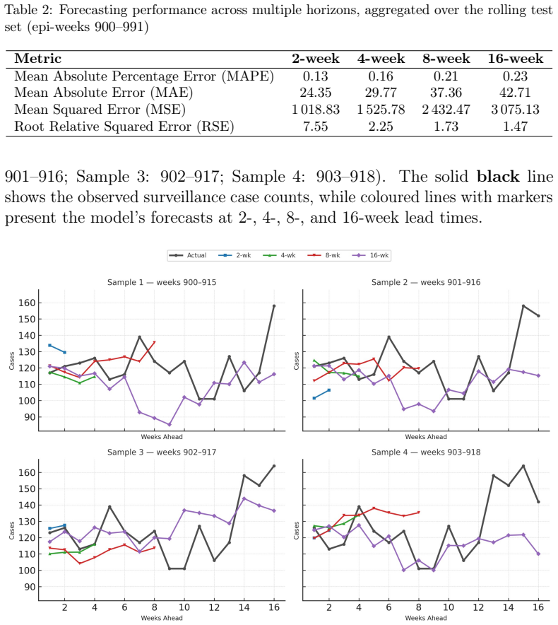
The central discovery is that relational structure among environmental predictors can carry Valley Fever forecasting: the GATv2-on-correlation-graph plus Transformer encoder-decoder reports MAPE of 0.13, 0.16, 0.21, and 0.23 for 2-, 4-, 8-, and 16-week horizons over test weeks 900-991, after training only through week 850. The feature gate selected the same 15 of roughly 190 variables in the top 10 percent across all four horizons, with 20-inch soil temperature maximum at lag 0 ranked first everywhere, followed by minimum relative humidity and six-week-lagged PM10. The paper interprets the stable selection and visual inspection of rolling 16-week samples as evidence that the model captures both short-term fluctuations and longer-term epidemiological trends, including the sharp rise around week 906.
Load-bearing premise
The load-bearing premise is that absolute Pearson correlations above 0.05, computed on original and six-week-lagged variables, capture the environmentally relevant dependencies; if the true relationships are nonlinear, nonstationary, or operate on longer lags, the network may be fitting noise or partial signals despite acceptable-looking test error.
Editorial extensions
If this is right
- At the 16-week horizon the model keeps MAPE at 0.23, so a health department could use it as a directional early-warning system, spotting rising or falling trends up to four months before cases arrive.
- Because 15 features rank in the top 10 percent at every horizon, the model identifies soil temperature, humidity, and PM10 as stable environmental drivers worth monitoring across seasons.
- The automatic feature gate reduces the input to 10 percent of variables, so the pipeline can be applied to new data without manual feature selection.
- The walk-forward evaluation protocol, with training ending at week 850 and testing on weeks 900-991 with fixed weights, provides an out-of-sample check across horizons, though it does not retrain the model during the test period.
Reading between the lines
- Editorial extension: a direct ablation that zeros all graph edges would reveal whether the graph structure, rather than the Transformer alone, is responsible for the forecast skill; the paper does not report such a comparison.
- Editorial extension: the paper tests only Maricopa County, so whether the same graph recipe transfers to Pima County or other endemic regions remains open; that transfer test is the natural next step.
- Editorial extension: the 0.05 correlation threshold and six-week lag cap are modeling choices, not tested results; sweeping both would show whether the identified features are stable or artifacts of the cutoff.
- Editorial extension: because no ARIMA or LSTM baseline appears in the experiments, "first successful implementation" is a novelty claim rather than a superiority claim; a head-to-head would put the MAPE values in context.
Editorial analysis
A structured set of objections, weighed in public.
Referee Report
Summary. The paper proposes a GNN-Transformer hybrid for forecasting weekly Valley Fever incidence in Maricopa County, Arizona. It constructs a variable graph from Pearson correlations thresholded at 0.05, includes lagged features up to six weeks, prunes inputs to the top 10% via a learned feature gate, applies GATv2 layers, and uses a Transformer encoder-decoder. The model is evaluated on forecast horizons of 2, 4, 8, and 16 weeks over epi-weeks 900-991, reporting MAPE between 0.13 and 0.23, MAE between 24.35 and 42.71, MSE between 1018.83 and 3075.13, and RSE between 7.55 and 1.47. The abstract and conclusion claim that the model effectively models Valley Fever trends, establishes the first successful graph-based deep learning approach for the disease, and provides early warning up to four months ahead.
Significance. The problem is practically relevant, and the authors provide code and data, a fixed-model walk-forward evaluation, and a 100-seed feature-importance stability analysis, all of which are commendable. If the reported accuracy were valid and supported by baselines, a variable-graph GNN could be a useful tool for public-health early warning. However, the evidence as presented does not support the headline claims: the RSE values contradict the other reported metrics under the standard definition, no baseline comparisons or error bars are provided, a 49-week gap exists between the training and test windows, and the claimed dynamic lag learning is not implemented. These issues are load-bearing because the paper's central contribution is the empirical forecasting claim.
major comments (5)
- [Section 4.5, Table 2] The RSE column is undefined, and the reported values contradict the other metrics under the standard definition. If RSE = sqrt(Σ(y-ŷ)² / Σ(y-ȳ)²), then every reported value exceeds 1, meaning the model is worse than always predicting the test-period mean. For the 2-week row, MSE=1018.83 gives RMSE≈31.9, so RSE=7.55 implies a mean-predictor RMSE of only ≈4.2, which is inconsistent with MAE=24.35 and MAPE=0.13 unless the metrics were computed on different scales or different samples. The paper must define RSE, report the test-period mean and variance, and provide at least mean, persistence, and standard time-series baselines; without this, the central claim of accurate forecasting is unsupported.
- [Section 4.3] The train/test split is under-specified. Training is described as including all weeks up to week 850, while testing is conducted on weeks 900-991, leaving 49 weeks (851-899) unaccounted for. If those weeks were excluded, the test period is not a simple continuation of the training window and the out-of-sample protocol changes; if they were used, the description is incorrect. This matters for the validity of the claimed out-of-sample performance, and the authors should explain why these weeks are missing or correct the description.
- [Sections 3.1 and 4.2] The method does not learn lag structures dynamically. Lagged features are generated only up to a fixed maximum of 6 weeks in Section 4.2, and the graph is built once from Pearson correlations thresholded at 0.05 in Section 3.1; no mechanism adapts the lag window or edge structure during training. The statement in Section 2.3 that graph architectures can learn optimal lag structures dynamically, and the conclusion's implication that the model captures critical delays through learned lagged effects, are therefore not supported by the implemented architecture. The authors should either implement an adaptive lag mechanism or explicitly temper these claims.
- [Sections 4.4 and 4.5] Forecast metrics are reported as point estimates from a single 92-week test window with no error bars or significance tests. The 100-seed analysis in Section 4.4 evaluates feature-importance stability only and does not quantify prediction uncertainty. The overlapping 16-week samples in Figure 4 (weeks 900-915, 901-916, 902-917, 903-918) are not independent, so the visual confirmation is weaker than it appears. The authors should report mean and standard deviation across seeds or bootstrap confidence intervals and test whether differences from baselines are statistically significant.
- [Section 4.5] There is no ablation isolating the contribution of the graph components. The paper does not compare the full model against ablated versions such as a Transformer without the graph module, a GAT without the feature gate, or a simple MLP using the same lagged features. Without such comparisons, the claimed benefits of the graph structure and feature selection cannot be evaluated, and the title claim of a 'Graph Neural Network approach' being responsible for the results is not established.
minor comments (6)
- [Author list] The affiliation line lists 'Hao Yana'; this is likely a typo for 'Hao Yan' and should be corrected.
- [Equation (9)] The reverse-differencing formula is written for h = 0, ..., H-1, which would reconstruct the target at time t for h=0; clarify whether the forecast horizon begins at t+1 and adjust the indexing accordingly.
- [Section 4.5] The sentence 'A forecasting model was trained on data from the in-sample period ending one epidemiological week prior to the rolling test set' is ambiguous about whether the model is retrained for each rolling window, while the next sentence says model weights remained fixed; state explicitly which protocol was used.
- [Figure 4] The four displayed 16-week samples are overlapping and therefore not independent evidence; the text should acknowledge this and avoid implying they are four separate validation checks.
- [References] The reference for the 2024 Arizona case count cites a non-peer-reviewed travel website (Vax-Before-Travel); the Arizona Department of Health Services or CDC primary data should be cited instead.
- [Acknowledgments] Grant DMS-1615879 is a National Science Foundation grant number, not an NIH grant; the acknowledgments should be corrected.
Circularity Check
No derivation-to-equivalence circularity; graph construction and normalization are applied over the full time series including the test window, so the reported 'out-of-sample' forecasts are partially informed by fitted inputs.
-
fitted input called prediction
[Section 3.1, graph construction (Pearson correlation and adjacency definition); cf. Section 4.3 train/test split.]
"Formally, let X = {xm,t} ∈ RM×T be the multivariate time series; the Pearson coefficient between series u and v is ρuv = (Σ_{t=1}^T (x_u,t − x̄_u)(x_v,t − x̄_v)) / (sqrt(Σ(x_u,t − x̄_u)^2) sqrt(Σ(x_v,t − x̄_v)^2)), and the adjacency weights are auv = |ρuv| if |ρuv| ≥ 0.05, 0 otherwise."
The adjacency weights are computed over the entire multivariate time series T with no stated restriction to the training window. Since the test period (weeks 900–991) is part of T, the graph structure used to encode variable relationships at test time is fitted using test-period values, including the target series. The model is then described as predicting those same weeks, so the reported errors are not strictly out-of-sample with respect to graph construction. The same full-series treatment is described for min-max normalization, which is applied to 'all features' without a train/test split. This is a fitted input that is presented as part of an independent forecast, rather than a forecast fully independent of the test data.
full rationale
The paper does not reduce its forecasting result to a fitted parameter: target values in weeks 900–991 are held out from weight training, and the model is evaluated with a rolling walk-forward protocol. There are no self-citations, no imported uniqueness theorems, and no ansatz smuggled in via citation. The central derivation—graph attention over correlation-based edges plus a Transformer encoder-decoder—is an independent machine-learning pipeline rather than a restatement of the data. The main circularity-adjacent issue is that graph adjacency and normalization are formally defined over the full time series without a training-only restriction, so the graph and scaling used at test time encode information from the forecast period. That is a leakage/fitted-input problem rather than a prediction that is equivalent to the target by construction, so it warrants a low score. The contradictory RSE values and the unexplained train/test gap are correctness and consistency concerns, not circularity, and would need separate resolution.
Assumptions & free parameters
free parameters (5)
- Lag window maximum =
6 weeks
- Correlation threshold =
0.05
- Feature retention rate =
0.10 (top 10%)
- Sequence length =
3 times forecast horizon
- Transformer dimensions =
256 embedding and feed-forward, 8 heads, dropout 0.05
assumptions (6)
- domain assumption Maricopa County ADHS surveillance counts accurately reflect true Valley Fever incidence over 2006-2024
- domain assumption AZMET and EPA point measurements represent county-wide environmental conditions
- ad hoc to paper Pearson correlation graph with threshold 0.05 captures the relevant dependency structure among variables and lagged features
- domain assumption A fixed maximum lag of 6 weeks is sufficient to capture environmental effects on incidence
- domain assumption First-order differencing makes the target stationary
- ad hoc to paper The test window (epi-weeks 900-991) is representative of future Valley Fever dynamics
Cite this review
Pith. "Pith review of Forecasting Coccidioidomycosis (Valley Fever) in Arizona: A Graph Neural Network Approach." pith.science (2026). https://pith.science/paper/LYGU5RLX
@misc{pith2026250710014,
  author       = {Pith},
  title        = {Pith review of: Forecasting Coccidioidomycosis (Valley Fever) in Arizona: A Graph Neural Network Approach},
  year         = {2026},
  howpublished = {\url{https://pith.science/paper/LYGU5RLX}},
  note         = {Machine review of arXiv:2507.10014}
}
read the original abstract
Coccidioidomycosis, commonly known as Valley Fever, remains a significant public health concern in endemic regions of the southwestern United States. This study develops the first graph neural network (GNN) model for forecasting Valley Fever incidence in Arizona. The model integrates surveillance case data with environmental predictors using graph structures, including soil conditions, atmospheric variables, agricultural indicators, and air quality metrics. Our approach explores correlation-based relationships among variables influencing disease transmission. The model captures critical delays in disease progression through lagged effects, enhancing its capacity to reflect complex temporal dependencies in disease ecology. Results demonstrate that the GNN architecture effectively models Valley Fever trends and provides insights into key environmental drivers of disease incidence. These findings can inform early warning systems and guide resource allocation for disease prevention efforts in high-risk areas.
Figures


Figures from the paper (1 more)
Reference graph
Works this paper leans on
-
[1]
Maricopa County . Valley fever, 2024. URL https://www.maricopa.gov/5813/Valley-Fever. Accessed: 2024-10-31
work page 2024
-
[2]
The public health impact of coccidioidomycosis in arizona and california
Richard F Hector, George W Rutherford, Clarisse A Tsang, Laura M Erhart, Orion McCotter, Shoana M Anderson, Kenneth Komatsu, Farzaneh Tabnak, Duc J Vugia, Ying Yang, et al. The public health impact of coccidioidomycosis in arizona and california. International journal of environmental research and public health, 8 0 (4): 0 1150--1173, 2011
work page 2011
-
[3]
Statistics for valley fever, 2024
Centers for Disease Control and Prevention . Statistics for valley fever, 2024. URL https://www.cdc.gov/valley-fever/php/statistics/index.html. Accessed: 2024-10-31
work page 2024
-
[4]
Infectious Diseases, Weather, and Climate
Philip M Polgreen and Evelyn L Polgreen. Infectious Diseases, Weather, and Climate . Clinical Infectious Diseases, 66 0 (6): 0 815--817, 12 2017. ISSN 1058-4838. doi:10.1093/cid/cix1105. URL https://doi.org/10.1093/cid/cix1105
-
[5]
Climate factors influencing coccidioidomycosis seasonality and outbreaks
Andrew C Comrie. Climate factors influencing coccidioidomycosis seasonality and outbreaks. Environmental health perspectives, 113 0 (6): 0 688--692, 2005
work page 2005
-
[6]
The habitat of coccidioides spp
Mar \' a del Roc \' o Reyes-Montes, Mar \' a Ameyali P \'e rez-Huitr \'o n, Jorge Luis Oca \ n a-Monroy, Mar \' a Guadalupe Fr \' as-De-Le \'o n, Erick Mart \' nez-Herrera, Roberto Arenas, and Esperanza Duarte-Escalante. The habitat of coccidioides spp. and the role of animals as reservoirs and disseminators in nature. BMC infectious diseases, 16: 0 1--8, 2016
work page 2016
-
[7]
Jennifer R Head, Gail Sondermeyer-Cooksey, Alexandra K Heaney, T Yu Alexander, Isabel Jones, Abinash Bhattachan, Simon K Campo, Robert Wagner, Whitney Mgbara, Sophie Phillips, et al. Effects of precipitation, heat, and drought on incidence and expansion of coccidioidomycosis in western usa: a longitudinal surveillance study. The Lancet Planetary Health, 6...
work page 2022
-
[8]
The endozoan, small-mammal reservoir hypothesis and the life cycle of coccidioides species
John W Taylor and Bridget M Barker. The endozoan, small-mammal reservoir hypothesis and the life cycle of coccidioides species. Medical Mycology, 57 0 (Supplement\_1): 0 S16--S20, 2019
work page 2019
Show all 34 references
-
[9]
Combining machine learning and conventional statistical approaches for risk factor discovery in a large cohort study
Iqbal Madakkatel, Ang Zhou, Mark D McDonnell, and Elina Hypp \"o nen. Combining machine learning and conventional statistical approaches for risk factor discovery in a large cohort study. Scientific reports, 11 0 (1): 0 22997, 2021
2021
-
[10]
Dobos, Kaitlin Benedict, Brendan R
Robert R. Dobos, Kaitlin Benedict, Brendan R. Jackson, and Orion Z. McCotter. Using soil survey data to model potential Coccidioides soil habitat and inform valley fever epidemiology. PLoS One, 16 0 (2): 0 e0247263, 2021. doi:10.1371/journal.pone.0247263
2021 doi
-
[11]
Relating coccidioidomycosis (valley fever) incidence to soil moisture conditions
EJ Coopersmith, JE Bell, K Benedict, J Shriber, O McCotter, and Michael H Cosh. Relating coccidioidomycosis (valley fever) incidence to soil moisture conditions. Geohealth, 1 0 (1): 0 51--63, 2017
2017
-
[12]
Enhanced surveillance for coccidioidomycosis, 14 us states, 2016
Kaitlin Benedict, Malia Ireland, Meghan P Weinberg, Randon J Gruninger, Jenna Weigand, Lei Chen, Katharine Perez-Lockett, Catherine Bledsoe, Lynn Denny, Katie Cibulskas, et al. Enhanced surveillance for coccidioidomycosis, 14 us states, 2016. Emerging infectious diseases, 24 0...
2016
-
[13]
Coccidioidomycosis incidence in arizona predicted by seasonal precipitation
James D Tamerius and Andrew C Comrie. Coccidioidomycosis incidence in arizona predicted by seasonal precipitation. PloS one, 6 0 (6): 0 e21009, 2011
2011
-
[14]
Valley fever: environmental risk factors and exposure pathways deduced from field measurements in california
Antje Lauer, Vicken Etyemezian, George Nikolich, Carl Kloock, Angel Franco Arzate, Fazalath Sadiq Batcha, Manpreet Kaur, Eduardo Garcia, Jasleen Mander, and Alyce Kayes Passaglia. Valley fever: environmental risk factors and exposure pathways deduced from field measurements in...
2020
-
[15]
Spatial scale in environmental risk mapping: A valley fever case study
Heidi E Brown, Mu Wangshu, Khan Mohammed, Tsang Clarisse, Liu Jian, and Tong Daoqin. Spatial scale in environmental risk mapping: A valley fever case study. Journal of Public Health Research, 6 0 (2): 0 jphr--2017, 2017
2017
-
[16]
Environmental factors affecting ecological niche of coccidioides species and spatial dynamics of valley fever in the united states
Elizabeth Weaver, Korine N Kolivras, R Quinn Thomas, Valarie A Thomas, and Kaja M Abbas. Environmental factors affecting ecological niche of coccidioides species and spatial dynamics of valley fever in the united states. Spatial and spatio-temporal epidemiology, 32: 0 100317, 2020
2020
-
[17]
Integrating artificial intelligence with mechanistic epidemiological modeling: a scoping review of opportunities and challenges
Yang Ye, Abhishek Pandey, Carolyn Bawden, Dewan Md Sumsuzzman, Rimpi Rajput, Affan Shoukat, Burton H Singer, Seyed M Moghadas, and Alison P Galvani. Integrating artificial intelligence with mechanistic epidemiological modeling: a scoping review of opportunities and challenges....
2025
-
[18]
A comprehensive survey on graph neural networks
Zonghan Wu, Shirui Pan, Fengwen Chen, Guodong Long, Chengqi Zhang, and S Yu Philip. A comprehensive survey on graph neural networks. IEEE transactions on neural networks and learning systems, 32 0 (1): 0 4--24, 2020
2020
-
[19]
Visitors at risk during arizona's valley fever outbreak, 2025
Vax-Before-Travel . Visitors at risk during arizona's valley fever outbreak, 2025. URL https://www.vax-before-travel.com/visitors-risk-during-arizonas-valley-fever-outbreak-2025-01-05. Reports Arizona Department of Health Services data: 14 , 680 Valley fever cases in Arizona f...
2025
-
[20]
Expansion of coccidioidomycosis endemic regions in the united states in response to climate change
Morgan E Gorris, Kathleen K Treseder, Charles S Zender, and James T Randerson. Expansion of coccidioidomycosis endemic regions in the united states in response to climate change. Geohealth, 3 0 (10): 0 308--327, 2019
2019
-
[21]
No consistent link between dust storms and valley fever (coccidioidomycosis)
AC Comrie. No consistent link between dust storms and valley fever (coccidioidomycosis). geohealth, 5, e2021gh000504, 2021
2021
-
[22]
Coccidioidomycosis (valley fever), soil moisture, and el nino southern oscillation in california and arizona
Kenneth J Tobin, Sugam Pokharel, and Marvin E Bennett. Coccidioidomycosis (valley fever), soil moisture, and el nino southern oscillation in california and arizona. International Journal of Environmental Research and Public Health, 19 0 (12): 0 7262, 2022
2022
-
[23]
Ferreira, Paula M
Marília I. Ferreira, Paula M. L. Correia, Elsa Pinto, et al. Hyperspectral imaging for the detection of plant pathogens in seeds: recent developments and challenges. Frontiers in Plant Science, 15: 0 1387925, 2024. doi:10.3389/fpls.2024.1387925. URL https://doi.org/10.3389/fpl...
2024
-
[24]
Machine learning at the edge for ai-enabled multiplexed pathogen detection
Vahid Ganjalizadeh, Gopikrishnan G Meena, Matthew A Stott, Aaron R Hawkins, and Holger Schmidt. Machine learning at the edge for ai-enabled multiplexed pathogen detection. Scientific Reports, 13 0 (1): 0 4744, 2023
2023
-
[25]
Transformehr: transformer-based encoder-decoder generative model to enhance prediction of disease outcomes using electronic health records
Zhichao Yang, Avijit Mitra, Weisong Liu, Dan Berlowitz, and Hong Yu. Transformehr: transformer-based encoder-decoder generative model to enhance prediction of disease outcomes using electronic health records. Nature communications, 14 0 (1): 0 7857, 2023
2023
-
[26]
Evaluating the effectiveness of self-attention mechanism in tuberculosis time series forecasting
Zhihong Lv, Rui Sun, Xin Liu, Shuo Wang, Xiaowei Guo, Yuan Lv, Min Yao, and Junhua Zhou. Evaluating the effectiveness of self-attention mechanism in tuberculosis time series forecasting. BMC Infectious Diseases, 24 0 (1): 0 1--13, 2024
2024
-
[27]
Covid-19 pandemic forecasting using cnn-lstm: a hybrid approach
Zuhaira M Zain and Nazik M Alturki. Covid-19 pandemic forecasting using cnn-lstm: a hybrid approach. Journal of Control Science and Engineering, 2021 0 (1): 0 8785636, 2021
2021
-
[28]
Predicting covid-19 disease progression and patient outcomes based on temporal deep learning
Chenxi Sun, Shenda Hong, Moxian Song, Hongyan Li, and Zhenjie Wang. Predicting covid-19 disease progression and patient outcomes based on temporal deep learning. BMC Medical Informatics and Decision Making, 21: 0 1--16, 2021
2021
-
[29]
Estimating the state of epidemics spreading with graph neural networks
Abhishek Tomy, Matteo Razzanelli, Francesco Di Lauro, Daniela Rus, and Cosimo Della Santina. Estimating the state of epidemics spreading with graph neural networks. Nonlinear Dynamics, 109 0 (1): 0 249--263, 2022
2022
-
[30]
Investigating the relationship between climate and valley fever (coccidioidomycosis)
Elizabeth A Weaver and Korine N Kolivras. Investigating the relationship between climate and valley fever (coccidioidomycosis). EcoHealth, 15: 0 840--852, 2018
2018
-
[31]
Review of remotely sensed data products for disease mapping and epidemiology
Sabelo Nick Dlamini, Anton Beloconi, Sizwe Mabaso, Penelope Vounatsou, Benido Impouma, and Ibrahima Soc \'e Fall. Review of remotely sensed data products for disease mapping and epidemiology. Remote Sensing Applications: Society and Environment, 14: 0 108--118, 2019
2019
-
[32]
Examining covid-19 forecasting using spatio-temporal graph neural networks
Amol Kapoor, Xue Ben, Luyang Liu, Bryan Perozzi, Matt Barnes, Martin Blais, and Shawn O'Banion. Examining covid-19 forecasting using spatio-temporal graph neural networks. arXiv preprint arXiv:2007.03113, 2020
2007 arXiv
-
[33]
Covid-19 infection inference with graph neural networks
Kyungwoo Song, Hojun Park, Junggu Lee, Arim Kim, and Jaehun Jung. Covid-19 infection inference with graph neural networks. Scientific reports, 13 0 (1): 0 11469, 2023
2023
-
[34]
A review of graph neural networks in epidemic modeling
Zewen Liu, Guancheng Wan, B Aditya Prakash, Max SY Lau, and Wei Jin. A review of graph neural networks in epidemic modeling. In Proceedings of the 30th ACM SIGKDD Conference on Knowledge Discovery and Data Mining, pages 6577--6587, 2024
2024
Reviewed August 6, 2026 · model on record in the stance chip above.
Discussion (0). Continue with ORCID to comment.