REVIEW 2 major objections 6 minor 28 references
A Mean Field Game for Capacity Expansion Modeling
T0 review · 2 major / 6 minor · reviewed 2026-08-06 · deepseek-v4-flash
Pith's one-line read The paper claims that in equilibrium, renewable producers invest only while their installed capacity sits below a time-dependent threshold, and that all investment ceases before the planning horizon ends.
desk verdict Finite-horizon capacity expansion MFG with a solid homogeneous part and a plausible heterogeneous extension that leans on an unquantified continuum approximation. read the letter →
The pith
A machine-rendered reading of the paper's core claim, the machinery that carries it, and where it could break.
The reading
What carries the argument
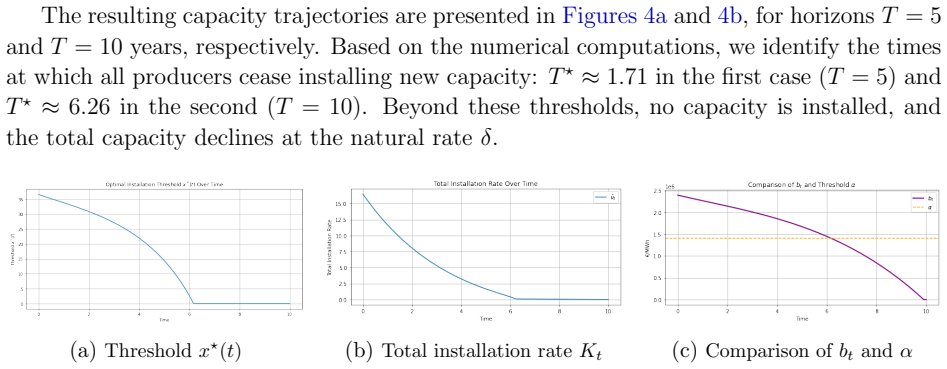
The load-bearing object is the threshold curve $x^\star(t)$, defined by $\partial V/\partial x(t,x^\star(t)) = \alpha + \beta N\bar\nu_t$ whenever the threshold is positive; here $V$ is the representative producer's value function, $\alpha$ the marginal installation cost, $\beta$ the crowding sensitivity, and $N\bar\nu_t$ the aggregate installation rate feeding back through the cost function. It separates a lower installation region, where producers add capacity, from an upper non-installation region, where capacity only decays and the value function has the closed form (26). The fixed-point condition (20) determines the mean installation rate from the density $m(t,x)$ and the value function, closing the mean field loop. In the homogeneous limit this same mechanism reduces to the adjoint variable $u_t$ crossing $\alpha$ once, which is the content of Lemma 3.3.
What would settle it
Simulate the finite-player game with $N=10$ and $N=100$ producers using the paper's linear-price parameters and compare the resulting aggregate investment trajectories and the time at which investment stops with the mean field equilibrium; if the discrepancy does not shrink as $N$ grows, the continuum approximation and the coupled HJB-FP characterization fail to describe the finite game.
Extended reading notes
Core claim
For a continuum of heterogeneous producers, the paper characterizes equilibrium by the coupled Hamilton-Jacobi-Bellman equation (18) and Fokker-Planck equation (19), joined through the mean capacity $\bar x_t$ and the mean installation rate $\bar\nu_t$. The optimal installation rate is $\nu^\star(t,x)=\frac{1}{2\beta}(\partial V/\partial x-\alpha-\beta N\bar\nu_t)^+$, so the value function's slope against the full marginal cost of installing capacity decides behavior. The authors show that, when revenue $xP(x+N\bar x)$ is concave in the producer's own capacity, the value function is concave and the optimal installation rate is non-increasing in capacity. Therefore the installation region is always an interval below a threshold $x^\star(t)$; producers at or above the threshold never invest, and in the homogeneous limit the critical time $T^\star$ is characterized by the adjoint variable $u_t$ crossing the marginal installation cost $\alpha$ exactly once (Lemma 3.3).
Load-bearing premise
The heterogeneous equilibrium requires that replacing true aggregate capacity and aggregate installation rate by their continuum averages is accurate, and the paper does not quantify how far that approximation is from the finite-player game.
Editorial extensions
If this is right
- With a Lipschitz price function the homogeneous forward-backward system has a unique solution, and under Assumption 3.1 there is a unique critical time $T^\star$ before which investment happens and after which capacity decays at rate $\delta$.
- For a linear price function, capacity follows a two-exponential formula during the investment phase, and the switch time solves a transcendental equation, so the threshold can be computed semi-explicitly.
- For heterogeneous producers, smaller producers invest at a higher rate than larger ones, and a producer whose capacity enters the non-installation region never invests again; all producers stop by a common terminal time $T^\star$.
- With stochastic capacity dynamics driven by geometric Brownian motion, the installation threshold is smaller than in the deterministic case, giving a precautionary slowdown in investment.
- For long planning horizons, the capacity path approaches the infinite-horizon steady state and stays near it until roughly 8.5 years before the terminal date in the reported parameter set.
Reading between the lines
- The paper leaves open the magnitude of the error in replacing finite aggregates by continuum means; a direct finite-player simulation would show how large the number of producers must be before the threshold structure becomes a good description.
- Because the threshold is pinned by the marginal cost of installation, policies that lower that cost or the crowding sensitivity would shift the investment window and the stopping time; this policy lever is present in the model but not developed.
- The same state-and-control mean field machinery likely applies to storage or other capacity-constrained green technologies with supply-chain congestion, although the paper does not claim this extension.
- The precautionary effect in the stochastic version suggests a testable prediction: measured uncertainty in renewable output should correlate with a later peak and a lower peak of aggregate investment, a comparison the paper does not run.
Signed reviews
Editorial analysis
A structured set of objections, weighed in public.
Referee Report
Summary. The paper develops a finite-horizon mean field game for capacity expansion in renewable electricity markets, in which producers interact through both the electricity price (a decreasing function of aggregate installed capacity) and the installation cost (increasing in the aggregate installation rate). In the homogeneous case, the game is reduced to a forward-backward ODE system (Eq. (6)); the paper proves existence and uniqueness, identifies a threshold time T* after which investment ceases, and gives a semi-explicit solution for a linear price function. In the heterogeneous case, the authors introduce a continuum aggregate approximation, derive a coupled HJB-FP system (Eqs. (18)-(19)), establish concavity of the value function and a threshold capacity x*(t), and propose two numerical methods for the linear-price and inverse-price specifications. A stochastic extension with idiosyncratic capacity shocks is also presented.
Significance. If the results are correct, the paper provides a useful and relatively tractable framework for studying strategic capacity expansion with crowding effects, and it extends the infinite-horizon model of [5] to finite horizons with heterogeneous producers. The homogeneous analysis is careful: Proposition 3.1 and Lemmas 3.3-3.4 give a reasonably complete picture of the forward-backward system, and the threshold/investment-stop structure is an appealing economic insight. The heterogeneous part is also transparent about its structural assumptions, and the numerical methods are cross-checked against each other. However, the paper's central heterogeneous claims rest on an unverified continuum approximation (Eq. (15)), and one displayed semi-explicit formula (the constant C in Proposition 3.2) appears to be incorrect. These issues need to be addressed before the paper can be recommended for publication.
major comments (2)
- [Section 3.2, Proposition 3.2] The constant C in Eq. (11) does not satisfy the stated boundary conditions. Solving X(0)=X0 and δX_T* + Xdot_T* = 0 for X = C e^{r1 t} + D e^{r2 t} + θ gives C = ((X0 - θ)(r2 + δ) + δθ e^{-r2 T*}) / ((r2 + δ) - e^{(r1-r2)T*}(r1 + δ)). The displayed formula instead has (X0 + θ)(r2 + δ) - δθ e^{-r2 T*} in the numerator. In the special case d2 = 0, one has r1 = r + δ and r2 = -δ, and the displayed formula yields C = +δθ e^{-(r+δ)T*}/(r + 2δ), whereas the boundary condition δX_T* + Xdot_T* = 0 requires C = -δθ e^{-(r+δ)T*}/(r + 2δ). This error propagates to Eq. (12) and to the claimed agreement between the shooting method and the semi-explicit solution in Figure 1b.
- [Section 4, Eq. (15)] The continuum aggregate approximation X_t ≈ x_t + N xbar_t and K_t ≈ ν_t + N νbar_t is the only bridge from the finite-player game (1)-(5) to the HJB-FP system (18)-(19). No error estimate for this approximation is provided, and the cited analysis [22] is listed as 'In preparation'. Since all heterogeneous results and the numerical experiments are formulated in this approximated game, the claims about the original finite-player model are conditional on an unverified approximation. The authors should either supply a quantitative error analysis (even for a restricted class of parameters or price functions) or explicitly restrict the paper's claims to the continuum aggregate game rather than to the N-player game.
minor comments (6)
- [Lemma 3.3, proof] The line 'implying Xt = X0 e^{-δt} > X0' has the inequality direction reversed; since K_s = 0 on [0,t], one has X_t = X0 e^{-δt} < X0. The subsequent comparison 0 ≤ dot u_t ≤ (r+δ)α - (P(X0)-c) is valid only with this corrected direction. The final sentence of the same proof should identify the actual contradiction: from dot u_t1 = dot u_t2 = 0 one obtains P(X_t1) = P(X_t2), hence X_t1 = X_t2, contradicting the strict decay X_t1 > X_t2.
- [Proposition 3.1, proof] After the Gronwall estimate, the displayed exponent (r + δ + hLM/(2β))T contains an unexplained factor 2. Applying Gronwall to Δ(T) ≤ Δ(0)e^{(r+δ)T} + (hLM/β)∫_0^T Δ(t) dt gives the constant hLM/β, not hLM/(2β). This is a typographical issue, but it should be corrected.
- [Section 4.3.2] The list of boundary conditions duplicates the 'at x = 0' bullet and writes 'at T = 0' where it should be 'at t = T'. The terminal condition for the value function should be imposed at the final time, not at T = 0.
- [Eq. (25)] The running reward f is written with hP(x_s + N xbar_s) - c, which is ambiguous; it should be h(P(x_s + N xbar_s) - c) so that the factor h multiplies both the price and the cost term.
- [Section 3.3, inverse price] Proposition 3.1 is stated for a globally Lipschitz price function P. The discussion of P(x) = p/x correctly notes that X_t is bounded away from zero and hence P is locally Lipschitz on the reachable set, but this should be formalized as a separate argument rather than asserted as 'effectively Lipschitz', because the proof of the comparison principle in Lemma 3.1 uses the global Lipschitz bound.
- [Section 4.2, definition of T*] The definition T* = inf{t : x*(s) = 0 for all s ∈ [t,T]} and the subsequent equalities x*(T*) = 0 and νbar_T* = 0 presume continuity of x* and νbar along the equilibrium. The paper does not state the regularity assumptions under which these properties hold; a brief regularity discussion or explicit assumptions would make the threshold characterization rigorous.
Circularity Check
No significant circularity: the equilibrium characterization and threshold results are derived from stated model primitives and explicit assumptions, not from fitted parameters or self-referential definitions.
full rationale
The paper's central claims are derived from the model primitives rather than from data fitting or self-referential definitions. In the homogeneous case, Proposition 3.1 proves existence and uniqueness of the forward-backward system (6a)-(6b) using standard ODE arguments, and Lemma 3.3 derives the threshold time T* from Assumption 3.1 and the monotonicity properties of the system; no fitted parameter is renamed as a prediction. In the heterogeneous case, the HJB-FP system (18)-(19) is obtained by writing the representative producer's optimization problem and the Fokker-Planck equation for the capacity distribution, and the threshold curve x*(t) follows from the concavity result in Lemma 4.1 and the explicit non-installation value function in Proposition 4.1 and Corollary 4.1. The numerical methods are validated against semi-explicit formulas and against each other, not against quantities that were used to calibrate the model. The only externally imported element is the continuum aggregate approximation (15), which is explicitly identified as an approximation used in prior work and whose error analysis is deferred to the authors' in-preparation reference [22]; this is an acknowledged modeling assumption rather than a circularly derived prediction, and the paper's theoretical results are stated conditionally on that approximation. No self-citation is used as a load-bearing uniqueness theorem or as a substitute for derivation, and no known empirical pattern is merely renamed. The paper is self-contained relative to its stated assumptions, so the circularity score is 0.
Assumptions & free parameters
assumptions (6)
- domain assumption The price function P is strictly decreasing.
- domain assumption P is Lipschitz continuous for the homogeneous existence and uniqueness result.
- ad hoc to paper Assumption 3.1: (P(X0)-c)h > (r+δ)α and there exists t0 with the discounted future price-minus-cost integral exceeding α.
- domain assumption The mapping x -> x P(x + N * x_bar) is concave.
- ad hoc to paper Continuum aggregate approximation X_t ≈ x_t + N * x_bar_t and K_t ≈ ν_t + N * ν_bar_t (Eq. (15)).
- domain assumption Existence and uniqueness of the coupled HJB-FP system (18)-(19).
Cite this review
Pith. "Pith review of A Mean Field Game for Capacity Expansion Modeling." pith.science (2026). https://pith.science/paper/QCS66UIR
@misc{pith2026250710604,
  author       = {Pith},
  title        = {Pith review of: A Mean Field Game for Capacity Expansion Modeling},
  year         = {2026},
  howpublished = {\url{https://pith.science/paper/QCS66UIR}},
  note         = {Machine review of arXiv:2507.10604}
}
read the original abstract
This paper studies the optimal investment behavior of renewable electricity producers in a competitive market, where both prices and installation costs are influenced by aggregate industry activity. We model the resulting crowding effects using a mean field game framework, capturing the strategic interactions among a continuum of heterogeneous producers. The equilibrium dynamics are characterized via a coupled system of Hamilton-Jacobi-Bellman and Fokker-Planck equations, which describe the value function of a representative producer and the evolution of the distribution of installed capacities over time. We analyze both deterministic and stochastic versions of the model, providing analytical insights in tractable cases and developing numerical methods to approximate the general solution. Simulation results illustrate how aggregate investment responds to changing market conditions, cost structures, and exogenous productivity shocks.
Figures


Figures from the paper (5 more)



Reference graph
Works this paper leans on
-
[5]
C. Alasseur, M. Basei, C. Bertucci, and A. Cecchin. A mean field model for the devel- opment of renewable capacities. Mathematics and Financial Economics , 17(4):695–719, 2023
work page 2023
- [22]
- [1]
- [2]
- [3]
-
[4]
C. Alasseur, I. Ben Taher, and A. Matoussi. An extended mean field game for storage in smart grids. Journal of Optimization Theory and Applications , 184(2):644–670, 2020
work page 2020
-
[6]
R. Bajo-Buenestado. The Iberian Peninsula blackout — Causes, consequences, and challenges ahead. Technical report, Rice University’s Baker Institute for Public Policy, 2025
work page 2025
-
[7]
A. Bassi` ere, R. Dumitrescu, and P. Tankov. A mean-field game model of electricity market dynamics. In F. E. Benth and A. E. D. Veraart, editors, Quantitative Energy Finance: Recent Trends and Developments , pages 181–219. Springer Nature Switzer- land, 2024
work page 2024
Show all 28 references
-
[8]
Bichuch, G
M. Bichuch, G. Dayanıklı, and M. Lauriere. A stackelberg mean field game for green regulator with a large number of prosumers. Preprint SSRN 4985557 , 2024
2024
-
[9]
Cacciarelli, P
D. Cacciarelli, P. Pinson, F. Panagiotopoulos, D. Dixon, and L. Blaxland. Do we actually understand the impact of renewables on electricity prices? A causal inference approach. Preprint arXiv:2501.10423, 2025
2025 arXiv
-
[10]
Carmona and M
R. Carmona and M. Ludkovski. Valuation of energy storage: an optimal switching approach. Quantitative Finance, 10(4):359–374, 2010
2010
-
[11]
Carmona and X
R. Carmona and X. Yang. Joint granular model for load, solar and wind power scenario generation. IEEE Transactions on Sustainable Energy , 15(1):674–686, 2024
2024
-
[12]
Carmona and C
R. Carmona and C. Zeng. Leveraging the turnpike effect for mean field games numerics. IEEE Open Journal of Control Systems , 3:389–404, 2024
2024
-
[13]
Carmona, G
R. Carmona, G. Dayanıklı, and M. Lauri` ere. Mean field models to regulate carbon emissions in electricity production. Dynamic Games and Applications , 12(3):897–928, 2022
2022
-
[14]
Carmona, G
R. Carmona, G. Dayanikli, F. Delarue, and M. Lauriere. From Nash equilibrium to social optimum and vice versa: a mean field perspective. Preprint arXiv:2312.10526 , 2023
2023 arXiv
-
[15]
Chan and R
P. Chan and R. Sircar. Fracking, renewables, and mean field games. SIAM Review, 59 (3):588–615, 2017. 29
2017
-
[16]
Dayanikli and M
G. Dayanikli and M. Lauri` ere. Multi-population mean field games with multiple major players: application to carbon emission regulations. In 2024 American Control Confer- ence, pages 5075–5081, 2024
2024
-
[17]
Dayanikli and M
G. Dayanikli and M. Lauriere. Cooperation, competition, and common pool resources in mean field games. Preprint arXiv:2504.09043, 2025
2025 arXiv
-
[18]
Dumitrescu, M
R. Dumitrescu, M. Leutscher, and P. Tankov. Energy transition under scenario uncer- tainty: a mean-field game of stopping with common noise. Mathematics and Financial Economics, 18(2):233–274, 2024
2024
-
[19]
´Elie, E
R. ´Elie, E. Hubert, T. Mastrolia, and D. Possama ¨ ı. Mean-field moral hazard for optimal energy demand response management. Mathematical Finance, 31(1):399–473, 2021
2021
-
[20]
Escribe, J
C. Escribe, J. Garnier, and E. Gobet. A mean field game model for renewable investment under long-term uncertainty and risk aversion. Dynamic Games and Applications , 14 (5):1093–1130, 2024
2024
-
[21]
Firoozi, A
D. Firoozi, A. V. Shrivats, and S. Jaimungal. Principal agent mean field games in REC markets. Preprint arXiv:2112.11963, 2022
2022 arXiv
-
[23]
Garcia, R
N. Garcia, R. Sircar, and M. Soner. Mean field games of control and cryptocurrency mining. Preprint, 2025
2025
-
[24]
Gu´ eant, J.-M
O. Gu´ eant, J.-M. Lasry, and P.-L. Lions. Mean field games and applications. In Paris-Princeton Lectures on Mathematical Finance 2010 , volume 2003, pages 205–266. Springer Berlin Heidelberg, Berlin, Heidelberg, 2011
2010
-
[25]
Hern´ andez Santib´ a˜ nez, A
N. Hern´ andez Santib´ a˜ nez, A. Jofr´ e, and D. Possama ¨ ı. Pollution regulation for electricity generators in a transmission network. SIAM Journal on Control and Optimization , 61 (2):788–819, 2023
2023
-
[26]
Z. Li, A. M. Reppen, and R. Sircar. A mean field games model for cryptocurrency mining. Management Science, 70(4):2188–2208, 2024
2024
-
[27]
Ludkovski and R
M. Ludkovski and R. Sircar. Technology ladders and R&D in dynamic Cournot markets. Journal of Economic Dynamics and Control , 69:127–151, 2016
2016
-
[28]
Shrivats, R
A. Shrivats, R. Sircar, and X. Yang. Quantifying renewables reliability risk in modern and future electric grids. The Journal of Energy Markets , 2024. To appear. 30
2024
Reviewed August 6, 2026 · model on record in the stance chip above.
Discussion (0). Continue with ORCID to comment.