REVIEW 3 major objections 5 minor 66 references
Granulation signatures in 3D hydrodynamical simulations: evaluating background model performance using a Bayesian nested sampling framework
T0 review · 3 major / 5 minor · reviewed 2026-08-06 · deepseek-v4-flash
Pith's one-line read Multi-component granulation models are consistently preferred over a single Harvey component across 27 convection simulations, with a tentative third component appearing beyond $\nu_{\mathrm{max}}$.
desk verdict Solid extension of Lundkvist+21 with a real Bayesian framework, but the model-ranking evidence—especially for the third component—rests on an untested subjective likelihood, so trust the broad multi-component result, not the details. read the letter →
The pith
A machine-rendered reading of the paper's core claim, the machinery that carries it, and where it could break.
The reading
What carries the argument
The load-bearing machinery is the mixed-model likelihood (Eq. 11): a granulation likelihood $L_1$, an exponential $\chi^2$ distribution with two degrees of freedom per frequency bin, is mixed with a constant-mean $\chi^2$ likelihood $L_2$ whose mean is fixed at 1% of the power near $\nu_{\mathrm{max}}$, with a sigmoid in frequency as the mixture coefficient so that power beyond $\nu_{\mathrm{max}}$ is progressively handed to $L_2$ and down-weighted. This lets the authors fit Harvey-profile models to the frequency range where granulation is visible in real stars while ignoring simulation-specific high-frequency artefacts. On top of that, nested sampling (Skilling 2004; Speagle 2020) with a convergence criterion of $\Delta \log Z = 0.1$ yields posterior samples and the evidence $Z$ for each model, and model comparisons reduce to evidence ratios with the prior odds set to 1. The four compared models are Harvey-type profiles: D has one amplitude, one characteristic frequency and one free exponent; J is the hybrid with a single amplitude but two characteristic frequencies; H has two independent components; and T adds a third, higher-frequency component.
What would settle it
Recompute all evidence ratios with the sigmoid transition moved to $0.5\nu_{\mathrm{max}}$ and to $2\nu_{\mathrm{max}}$ while keeping everything else fixed; if the preference for the three-component model beyond $\nu_{\mathrm{max}}$ reverses or vanishes, that component is a product of the weighting rather than an intrinsic granulation feature. A second check is to refit the solar spectrum with a more realistic oscillation-envelope model, such as a Voigt profile or an explicit mode list, and see whether the strong preference for the three-component model survives.
Extended reading notes
Core claim
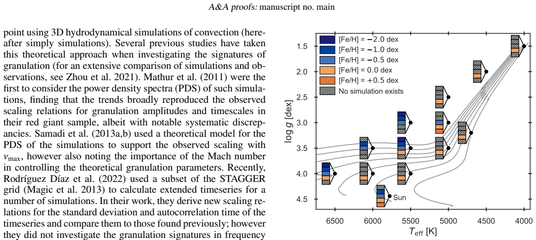
The authors claim that, judged by Bayesian evidence, a single Harvey-type background component never wins: across the full simulation suite the hybrid model J (one amplitude, two characteristic frequencies), the two-component model H, and the three-component model T each outperform the single-component model D, with J preferred for most simulations and T preferred for several, including the near-noise-free Sun. Because the simulations contain no magnetic activity, the consistent preference for a second component cannot be attributed to stellar faculae, which had been proposed as the source of the second component in observations. The paper further claims a tentative third granulation component beyond $\nu_{\mathrm{max}}$ for numerous simulations, explicitly cautioning that it could be either a genuine high-frequency granulation signature or a product of numerical box-mode harmonics; and that in the Sun the three-component model is very strongly preferred, while for KIC 8006161 the two- and three-component models are statistically comparable. A direct corollary is that the recovered exponents of all components exceed the literature expectations of about 4, and that the inferred $\nu_{\mathrm{max}}$ shifts with the chosen background model, so background descriptions feed directly into asteroseismic parameter estimation.
Load-bearing premise
Every reported model preference, including the tentative third component, is computed under a deliberately subjective likelihood weighting: above $\nu_{\mathrm{max}}$ a sigmoid fades the granulation likelihood out and hands the fit to a flat $\chi^2$ distribution whose mean is fixed at 1% of the power near $\nu_{\mathrm{max}}$, so changing the transition frequency or that 1% can change the evidence ratios and the conclusions built on them.
Editorial extensions
If this is right
- Single-component background descriptions should be considered insufficient for granulation in solar-like stars, since a multi-component model is preferred for every simulation in the suite.
- Stellar faculae are not the sole source of the second granulation component, because the activity-free simulations show the same preference for two or more components.
- A third granulation component beyond $\nu_{\mathrm{max}}$ is tentatively present in some simulations and possibly in the Sun, but verifying it in typical observations requires a better model of the oscillation excess than the Gaussian envelope used here.
- The recovered $\nu_{\mathrm{max}}$ depends on which background model is fitted, so the choice of background description propagates into asteroseismic parameter estimates such as surface gravity and radius.
- Total granulation amplitudes recovered from the simulations scale with $\nu_{\mathrm{max}}$ as power laws with slopes near $-0.52$, offset from the observed relation, showing that derived granulation parameters depend on both the dataset and the chosen model.
Reading between the lines
- Re-running the evidence comparison with the sigmoid transition placed at $0.5\nu_{\mathrm{max}}$ or $2\nu_{\mathrm{max}}$, or with the constant likelihood mean set to a different fraction of the power, would test whether the third-component preference is a genuine feature or an artefact of where the weighting drops.
- Fitting the same simulations at different numerical resolutions or Mach numbers would tell whether the tentative third component tracks box-mode harmonics; if it moves with resolution, it is numerical rather than granulation.
- The sigmoid transition is anchored to the same $\nu_{\mathrm{max}}$ whose value the background model influences; treating the transition frequency as an uncertain fitted parameter would be a stronger test of the beyond-$\nu_{\mathrm{max}}$ component.
- Connecting the two-component preference to the bimodal granule-size distribution documented for this class of simulations suggests a route to a physically motivated background model, which the paper leaves as future work.
Editorial analysis
A structured set of objections, weighed in public.
Referee Report
Summary. The manuscript compares four parametric descriptions of the granulation background—a single Harvey component (D), a hybrid two-timescale model (J), a two-component model (H), and a three-component model (T)—by fitting power density spectra of 27 non-magnetic 3D hydrodynamical convection simulations from Rodríguez Díaz et al. (2022). Model comparison is performed with a Bayesian nested-sampling framework (Dynesty) under the mixed-model likelihood of Eq. (11), and the framework is then applied to KIC 8006161 and VIRGO solar data. The main findings are that multi-component models are consistently preferred over the single-component model, that the hybrid model J performs well for many simulations, and that a tentative third component beyond νmax is seen for some simulations; the paper also reports granulation amplitude and characteristic-frequency scaling relations and finds exponents steeper than expected.
Significance. If the model-preference results are robust, this is a valuable contribution: it extends granulation-background model tests to a broad HR-diagram suite of simulations without observational noise, provides a public nested-sampling framework, and sharpens the debate on whether multi-component granulation backgrounds are needed. The conclusion that faculae cannot be the sole source of the second component is well motivated because the simulations are non-magnetic. However, the significance is currently conditional: the evidence ratios are computed with a subjective fractional likelihood whose tuning parameters are not specified or tested, and the model J amplitude prior is partly derived from the same simulations, so the exact strengths and rankings of the preferences are not yet established. The paper is transparent about the main confounders for the third component, which is a strength, but the wording in Sect. 4.1 is somewhat stronger than the evidence supports.
major comments (3)
- [§3.2, Eq. (11)] The mixed-model likelihood is not a proper sampling distribution for the PDS, and the two subjective ingredients are underspecified and untested. L2 is fixed to a χ2 distribution with constant mean equal to 1% of the power near νmax, and p(ν) is described only as a sigmoid whose 'plateau and slope' are set from νmax, with no explicit functional form. Since every log-evidence difference in Fig. 4 and Tables 3 and C.1 is computed from Eq. (11), the entire model ranking is conditional on these choices. The concern is most acute for model T, whose third component lies beyond νmax where p(ν) has decayed and L2 has increasing weight; a moderate change in sigmoid width or in the L2 mean could alter or erase the preference for T. I ask the authors to (i) state the exact sigmoid parameterization, and (ii) repeat the model comparison for a small grid of transition frequencies, sigmoid widths, and L2 mean levels (for example 0.1%, 1%, and 10% of the power near νmax), reporting how the rankings in Fig. 4 change. Without this, the Jeffreys-scale interpretation of |Δlog Z| is not calibrated.
- [Appendix B, Table B.2] The prior for the model J amplitude is derived from preliminary fits to the same simulation suite: the text states that 'we derived our own scaling relation for its amplitude' after 'running test-fits with wide priors' on these simulations. This makes the J evidence a within-sample quantity; the J-versus-H and J-versus-T comparisons in Fig. 4 are therefore not fully out-of-sample Bayes factors and may be biased in J's favor. The D-versus-multi-component conclusion is less affected because D's prior is anchored to Kallinger et al. (2014), but the specific ranking of J relative to H and T needs to be re-examined. A practical remedy would be to calibrate the J amplitude prior on one subset of the simulations and evaluate on the complementary subset, or to show that using the Kallinger et al. (2014) prior with a wider σ leaves the J-versus-H/T evidence ratios qualitatively unchanged.
- [§4.1, Fig. 7, and §7] The tentative third component is inferred from the evidence for model T and from the apparent scaling of its characteristic frequency f with νmax. The paper itself notes in §4.1 that the simulation box modes and their harmonics also scale with νmax, so the scaling of f is not a discriminating test. The sentence in §4.1 ('This is interesting and suggests the presence of a genuine granulation component beyond νmax') is stronger than the evidence supports, given that the box modes were artificially damped and residual harmonics are a plausible alternative explanation. I recommend either softening this sentence or adding a concrete diagnostic, such as comparing fits to simulations with and without box-mode damping or checking the third-component frequency against known harmonic frequencies, so that the claim is presented as a testable hypothesis rather than a tentative detection.
minor comments (5)
- [§3.2] The sigmoid function should be written out explicitly, including how its midpoint and width depend on νmax; referring only to 'plateau and slope' is insufficient for reproducibility.
- [Fig. 4] Because the colorbar saturates at |Δlog Z| ≳ 10, the differences among 'overwhelming' preferences are not visible in the figure; a supplementary table with all numerical evidence ratios would make the results more usable.
- [Data availability] The text says the fitting framework is accessible on GitHub but gives no URL or version identifier; a permanent repository link or DOI should be supplied.
- [Table C.1] The entry '2542 .57' contains an unintended space between the integer and decimal part; this should be corrected.
- [§6.1] The statement that the simulations 'rule out' stellar faculae as the sole source of the second component is slightly overstrong, since simulations also lack other real-star complications; 'argue against' would be more precise, although the non-magnetic nature of the simulations is indeed a strong argument.
Circularity Check
The J-amplitude prior is fitted to the same simulation suite on which J is then preferred, and the reported agreement with Kallinger scalings is partly prior echo; the central multi-component preference still has independent support from H and T.
-
fitted input called prediction
[Appendix B (prior derivation for model J) applied in Sect. 4 (Fig. 4) and Sect. 4.1 (Fig. 6)]
"As model J takes a different shape than the rest, we derived our own scaling relation for its amplitude. This was done by first running test-fits with wide priors set by the scaling relations of Kallinger et al. (2014), before deriving a scaling relation for the amplitude based on the preliminary outcomes, and subsequently using it when producing the results of this work."
The lognormal prior for the J amplitude (Table B.2) is derived from preliminary fits to the same simulation suite whose PDS are then used to compute the evidence ratios in Fig. 4. Model J's preference over D, H, and T is therefore not a fully out-of-sample Bayes factor: part of its support is inherited from a prior tuned to the data being compared. Similarly, the posterior amplitude scaling for J in Fig. 6 is anchored to a relation fitted on the same data, so the recovered values and the fitted power law are partly the same input returned as output. This does not by itself force the D-versus-multi conclusion, since models H and T use externally anchored priors and are also preferred over D.
-
self definitional
[Sect. 3.4 (priors) and Sect. 4.1 (scaling results), with Table B.2]
"Sect. 3.4: 'Kallinger et al. (2014) derived various scaling relations for the granulation amplitudes and characteristic frequencies in their work, which we generally rely on to inform our priors, with certain nuances depending on the model (see Appendix B).' Sect. 4.1: 'generally follow the observationally determined scaling from Kallinger et al. (2014).'"
The amplitudes and characteristic frequencies in Figs. 6 and 7 are sampled with lognormal priors whose means are set by the Kallinger et al. (2014) power laws (Table B.2). Claiming in Sect. 4.1 that the recovered values 'generally follow' Kallinger et al. is therefore partly a restatement of the prior input rather than an independent confirmation. The comparison retains some independent content because the fitted power-law slopes (e.g., s = -0.516 ± 0.005 for J) differ from Kallinger's -0.564 ± 0.002, but the agreement claim is weaker than presented.
full rationale
Most of the paper is a self-contained model-comparison exercise: the evidence ratios in Fig. 4 and Tables 3 and C.1 are computed from the PDS via Eqs. 9-11, and the central result that multi-component models are preferred over the single-component D model does not reduce to any input by construction. Models H and T beat D under priors anchored to the external Kallinger et al. (2014) scalings, so that conclusion is data-driven. The circularity concerns are limited to two places. First, the amplitude prior for model J was fitted to preliminary runs on the same simulation suite (Appendix B), so the J-specific evidence and the J amplitude scaling in Figs. 4 and 6 are partly inherited from the prior, making J's comparisons not fully out-of-sample. Second, the reported agreement of the recovered amplitudes and characteristic frequencies with Kallinger scaling in Sect. 4.1 is partly prior echo, because the priors in Table B.2 are centered on those same Kallinger power laws; the differing fitted slopes show this is not entirely forced. The mixed-model likelihood (Eq. 11) is an acknowledged subjective weighting whose sigmoid transition and constant high-frequency mean are not tested in a sensitivity analysis; this is a robustness limitation for the tentative beyond-νmax third-component claim, but it is not circularity, since the third component is fitted from the data and the weighting is not derived from the conclusion. Self-citations to Lundkvist et al. (2021) motivate model J, but the model is re-tested here on new data and is not used as an unverified uniqueness argument, so they are not load-bearing. Overall, the central multi-component preference has independent support, while the J-specific evidence and the scaling 'agreement' are partially circular.
Assumptions & free parameters
free parameters (7)
- Granulation component amplitudes a, c, e =
see Fig. 6
- Characteristic frequencies b, d, f =
see Fig. 7
- Exponents l, k, m =
Table 2 medians
- L2 constant mean for mixed-model likelihood =
1% of power near νmax
- Sigmoid weighting parameters =
set from νmax
- Model J amplitude prior scaling constants =
derived from preliminary test fits
- Total amplitude power-law constants k, s =
k=3040-3140; s=-0.515 to -0.522
assumptions (6)
- domain assumption Power density spectrum bins follow a χ2 distribution with 2 degrees of freedom
- domain assumption Granulation background is a sum of Harvey/super-Lorentzian components
- domain assumption Box modes have been removed from simulation timeseries
- ad hoc to paper The sigmoid mixture likelihood is a valid likelihood for model evidence
- domain assumption Oscillation excess is Gaussian (Eq. 3)
- standard math Bayes factor evidence from Dynesty with Δlog Z=0.1 is converged
invented entities (1)
-
Third granulation component (model T)
Cite this review
Pith. "Pith review of Granulation signatures in 3D hydrodynamical simulations: evaluating background model performance using a Bayesian nested sampling framework." pith.science (2026). https://pith.science/paper/LN72L55L
@misc{pith2026250711699,
  author       = {Pith},
  title        = {Pith review of: Granulation signatures in 3D hydrodynamical simulations: evaluating background model performance using a Bayesian nested sampling framework},
  year         = {2026},
  howpublished = {\url{https://pith.science/paper/LN72L55L}},
  note         = {Machine review of arXiv:2507.11699}
}
abstract
Understanding the granulation background signal is of vital importance when interpreting the asteroseismic diagnostics of solar-like oscillators. Various descriptions exist in the literature for modelling the surface manifestation of convection, the choice of which affects our interpretations. We aim to evaluate the performance of and preference for various granulation background models for a suite of 3D hydrodynamical simulations of convection across the HR diagram, thereby expanding the number of simulations and coverage of parameter space for which such studies have been made. We take a statistical approach by considering the granulation in power density spectra of 3D simulations, where no biases or systematics of observational origin are present. To properly contrast the performance of the models, we develop a Bayesian nested sampling framework for model inference and comparison. This framework was extended to real stellar data using KIC 8006161 (Doris) and the Sun. We find that multi-component models are consistently preferred over a single-component model, with each tested multi-component model demonstrating merit in specific cases. This occurs for simulations with no magnetic activity, thus ruling out stellar faculae as the sole source of the second granulation component. Like a previous study, we find that a hybrid model with a single overall amplitude and two characteristic frequencies performs well for numerous simulations. Additionally, a tentative third granulation component beyond the value of $\nu_\mathrm{max}$ is seen for some simulations, but its potential presence in observations requires further efforts. Studying the granulation signatures in these simulations paves the way to studying stars with accurate granulation models. This deeper understanding of the granulation signal may lead to complementary methods to existing algorithms for determining stellar parameters.
Figures


Figures from the paper (7 more)


Reference graph
Works this paper leans on
-
[1]
, " * write output.state after.block = add.period write newline
ENTRY address archiveprefix author booktitle chapter edition editor howpublished institution eprint journal key month note number organization pages publisher school series title type volume year label extra.label sort.label short.list INTEGERS output.state before.all mid.sentence after.sentence after.block FUNCTION init.state.consts #0 'before.all := #1 ...
-
[2]
write newline
" write newline "" before.all 'output.state := FUNCTION n.dashify 't := "" t empty not t #1 #1 substring "-" = t #1 #2 substring "--" = not "--" * t #2 global.max substring 't := t #1 #1 substring "-" = "-" * t #2 global.max substring 't := while if t #1 #1 substring * t #2 global.max substring 't := if while FUNCTION word.in bbl.in " " * FUNCTION format....
-
[3]
R., Duvall , Thomas L., J., & Jefferies , S
Anderson , E. R., Duvall , Thomas L., J., & Jefferies , S. M. 1990, , 364, 699
1990
- [4]
-
[5]
Ballot , J., Barban , C., & van't Veer-Menneret , C. 2011, , 531, A124
work page 2011
-
[6]
Bastien , F. A., Stassun , K. G., Basri , G., & Pepper , J. 2016, , 818, 43
work page 2016
-
[7]
Bedding , T. R. 2014, in Asteroseismology, ed. P. L. Pall \'e & C. Esteban , 60
work page 2014
-
[8]
1958, , 46, 108
B \"o hm-Vitense , E. 1958, , 46, 108
1958
Show all 66 references
-
[9]
J., Koch , D., Basri , G., et al
Borucki , W. J., Koch , D., Basri , G., et al. 2010, Science, 327, 977
2010
-
[10]
A., Davies , G
Bugnet , L., Garc \' a , R. A., Davies , G. R., et al. 2018, , 620, A38
2018
-
[11]
D., & Pereyra , M
Cai , X., McEwen , J. D., & Pereyra , M. 2021, arXiv e-prints, arXiv:2106.03646
2021 arXiv
-
[12]
L., Chaplin , W
Campante , T. L., Chaplin , W. J., Lund , M. N., et al. 2014, , 783, 123
2014
-
[13]
J., Bedding , T
Chaplin , W. J., Bedding , T. R., Bonanno , A., et al. 2011 a , , 732, L5
2011
-
[14]
J., Kjeldsen , H., Bedding , T
Chaplin , W. J., Kjeldsen , H., Bedding , T. R., et al. 2011 b , , 732, 54
2011
-
[15]
Chaplin , W. J. & Miglio , A. 2013, , 51, 353
2013
-
[16]
A., et al
Corsaro , E., Mathur , S., Garc \' a , R. A., et al. 2017, , 605, A3
2017
-
[17]
G., Pratt , J., Vlaykov , D
Dethero , M. G., Pratt , J., Vlaykov , D. G., et al. 2024, , 692, A46
2024
-
[18]
2024, The Open Journal of Astrophysics, 7, 79
Dittmann , A. 2024, The Open Journal of Astrophysics, 7, 79
2024
-
[19]
G., et al
Freytag , B., Steffen , M., Ludwig , H. G., et al. 2012, Journal of Computational Physics, 231, 919
2012
-
[20]
N., Berthomieu , G., et al
Froehlich , C., Andersen , B. N., Berthomieu , G., et al. 1988, VIRGO: The solar monitor experiment on SOHO , In ESA, The SOHO Mission. Scientific and Technical Aspects of the Instruments p 19-23 (SEE N90-13302 04-92)
1988
-
[21]
2020, arXiv e-prints, arXiv:2011.01808
Gelman , A., Vehtari , A., Simpson , D., et al. 2020, arXiv e-prints, arXiv:2011.01808
2020 arXiv
-
[22]
& Campante , T
Handberg , R. & Campante , T. L. 2011, , 527, A56
2011
-
[23]
& Lund , M
Handberg , R. & Lund , M. N. 2014, , 445, 2698
2014
-
[24]
1985, in ESA Special Publication, Vol
Harvey , J. 1985, in ESA Special Publication, Vol. 235, Future Missions in Solar, Heliospheric & Space Plasma Physics, ed. E. Rolfe & B. Battrick , 199
1985
-
[25]
2009, , 506, 465
Hekker , S., Kallinger , T., Baudin , F., et al. 2009, , 506, 465
2009
-
[26]
2024, arXiv e-prints, arXiv:2403.02489
Hey , D., Huber , D., Ong , J., Stello , D., & Foreman-Mackey , D. 2024, arXiv e-prints, arXiv:2403.02489
2024 arXiv
-
[27]
A., Hanslmeier , A., & Sobotka , M
Hirzberger , J., V \'a zquez , M., Bonet , J. A., Hanslmeier , A., & Sobotka , M. 1997, , 480, 406
1997
-
[28]
R., Stello , D., et al
Huber , D., Bedding , T. R., Stello , D., et al. 2011, , 743, 143
2011
-
[29]
& Roos, M
James, F. & Roos, M. 1975, Comput. Phys. Commun., 10, 343
1975
-
[30]
1961, Theory of Probability , 3rd edn
Jeffreys , H. 1961, Theory of Probability , 3rd edn. (Oxford University Press)
1961
-
[31]
2014, , 570, A41
Kallinger , T., De Ridder , J., Hekker , S., et al. 2014, , 570, A41
2014
-
[32]
L., Ballot , J., et al
Karoff , C., Campante , T. L., Ballot , J., et al. 2013, , 767, 34
2013
-
[33]
2013, Stellar Structure and Evolution
Kippenhahn , R., Weigert , A., & Weiss , A. 2013, Stellar Structure and Evolution
2013
-
[34]
& Bedding , T
Kjeldsen , H. & Bedding , T. R. 2011, , 529, L8
2011
-
[35]
1991, , 250, 50
Krishan , V. 1991, , 250, 50
1991
-
[36]
2002, , 334, 230
Krishan , V., Paniveni , U., Singh , J., & Srikanth , R. 2002, , 334, 230
2002
-
[37]
R., Huber , D., et al
Li , Y., Bedding , T. R., Huber , D., et al. 2024, , 974, 77
2024
-
[38]
Littenberg , T. B. & Cornish , N. J. 2015, , 91, 084034
2015
-
[39]
Ludwig , H. G. 2006, , 445, 661
2006
-
[40]
N., Silva Aguirre , V., Davies , G
Lund , M. N., Silva Aguirre , V., Davies , G. R., et al. 2017, , 835, 172
2017
-
[41]
S., Ludwig , H.-G., Collet , R., & Straus , T
Lundkvist , M. S., Ludwig , H.-G., Collet , R., & Straus , T. 2021, , 501, 2512
2021
- [42]
-
[43]
2013, , 557, A26
Magic , Z., Collet , R., Asplund , M., et al. 2013, , 557, A26
2013
-
[44]
2011, , 741, 119
Mathur , S., Hekker , S., Trampedach , R., et al. 2011, , 741, 119
2011
-
[45]
M., et al
Mathur , S., Huber , D., Batalha , N. M., et al. 2017, , 229, 30
2017
-
[46]
2009, , 495, 979
Michel , E., Samadi , R., Baudin , F., et al. 2009, , 495, 979
2009
-
[47]
D., Romeijn, J.-W., & Rouder, J
Morey, R. D., Romeijn, J.-W., & Rouder, J. N. 2016, Journal of Mathematical Psychology, 72, 6, bayes Factors for Testing Hypotheses in Psychological Research: Practical Relevance and New Developments
2016
-
[48]
2021, , 647, A168
M \"u llner , M., Zwintz , K., Corsaro , E., et al. 2021, , 647, A168
2021
-
[49]
& Stein , R
Nordlund , A . & Stein , R. F. 2001, , 546, 576
2001
-
[50]
2024, arXiv e-prints, arXiv:2406.05447
Rauer , H., Aerts , C., Cabrera , J., et al. 2024, arXiv e-prints, arXiv:2406.05447
2024 arXiv
-
[51]
R., Winn , J
Ricker , G. R., Winn , J. N., Vanderspek , R., et al. 2014, in Society of Photo-Optical Instrumentation Engineers (SPIE) Conference Series, Vol. 9143, Space Telescopes and Instrumentation 2014: Optical, Infrared, and Millimeter Wave, ed. J. Oschmann , Jacobus M., M. Clampin , ...
2014
-
[52]
F., Bigot, L., Aguirre Børsen-Koch, V., et al
Rodríguez Díaz, L. F., Bigot, L., Aguirre Børsen-Koch, V., et al. 2022, Monthly Notices of the Royal Astronomical Society, 514, 1741
2022
-
[53]
Samadi , R., Belkacem , K., & Ludwig , H. G. 2013 a , , 559, A39
2013
-
[54]
G., et al
Samadi , R., Belkacem , K., Ludwig , H. G., et al. 2013 b , , 559, A40
2013
-
[55]
2019, , 624, A117
Samadi , R., Deru , A., Reese , D., et al. 2019, , 624, A117
2019
-
[56]
1949, Proceedings of the IRE , 37, 10
Shannon, C. 1949, Proceedings of the IRE , 37, 10
1949
-
[57]
2004, in American Institute of Physics Conference Series, Vol
Skilling , J. 2004, in American Institute of Physics Conference Series, Vol. 735, Bayesian Inference and Maximum Entropy Methods in Science and Engineering: 24th International Workshop on Bayesian Inference and Maximum Entropy Methods in Science and Engineering, ed. R. Fischer...
2004
-
[58]
Speagle , J. S. 2020, , 493, 3132
2020
-
[59]
R., Bedding , T
Sreenivas , K. R., Bedding , T. R., Huber , D., et al. 2025, , 537, 3265
2025
-
[60]
R., Bedding , T
Sreenivas , K. R., Bedding , T. R., Li , Y., et al. 2024, , 530, 3477
2024
-
[61]
J., Basu , S., Elsworth , Y., & Bedding , T
Stello , D., Chaplin , W. J., Basu , S., Elsworth , Y., & Bedding , T. R. 2009, , 400, L80
2009
-
[62]
2006, , 369, 2025
Tepper-Garc \' a , T. 2006, , 369, 2025
2006
-
[63]
Trampedach , R., Christensen-Dalsgaard , J., Nordlund , A., & Stein , R. F. 1998, in The First MONS Workshop: Science with a Small Space Telescope, ed. H. Kjeldsen & T. R. Bedding , 59
1998
-
[64]
F., Christensen-Dalsgaard , J., Nordlund , A ., & Asplund , M
Trampedach , R., Stein , R. F., Christensen-Dalsgaard , J., Nordlund , A ., & Asplund , M. 2014, , 445, 4366
2014
-
[65]
R., et al
Yu , J., Huber , D., Bedding , T. R., et al. 2018, , 236, 42
2018
-
[66]
2021, , 503, 13
Zhou , Y., Nordlander , T., Casagrande , L., et al. 2021, , 503, 13
2021
Reviewed August 6, 2026 · model on record in the stance chip above.
Discussion (0). Sign in to comment.