REVIEW 4 major objections 6 minor 17 references
Physics constrained learning of stochastic characteristics
T0 review · 4 major / 6 minor · reviewed 2026-08-06 · deepseek-v4-flash
Pith's one-line read Adding innovation-consistency terms to the training loss improves vehicle state estimation by producing more accurate noise covariances.
desk verdict New loss terms for learning Q and R; the experimental support is thinner than the claim, but a legitimate preliminary study. read the letter →
The pith
A machine-rendered reading of the paper's core claim, the machinery that carries it, and where it could break.
The reading
What carries the argument
The load-bearing object is the innovation sequence, $\nu_k = z_k - H \hat{x}_k^-$, and the two optimality statistics built from it: the time-averaged innovation autocorrelation matrix $\hat{C}_i$ and the time-averaged normalized innovation square $\bar{\epsilon}_\nu$. An optimal Kalman filter has white innovations, so the autocorrelation should vanish for nonzero lags and the normalized innovation square should average to one; the paper converts these statistical conditions into penalty terms in the LSTM training loss. The learned map is an LSTM fed with a length-100 sequence of measurements and innovations together with the previous Q and R estimates, and its output supplies the two process-noise variances and the measurement-noise variance to the filter at each step. These constraints do the argument's work because they tie the predicted noise statistics to the filter's own consistency, which is the condition that an incorrectly chosen covariance would violate.
What would settle it
Generate simulated trajectories with Qa swept across a grid while Qb and R are held fixed, and check whether the LSTM's predicted Qa tracks the true value; if it does not and the final state RMSE still improves, the claimed mechanism (better covariance identification) is not what drives the improvement.
Extended reading notes
Core claim
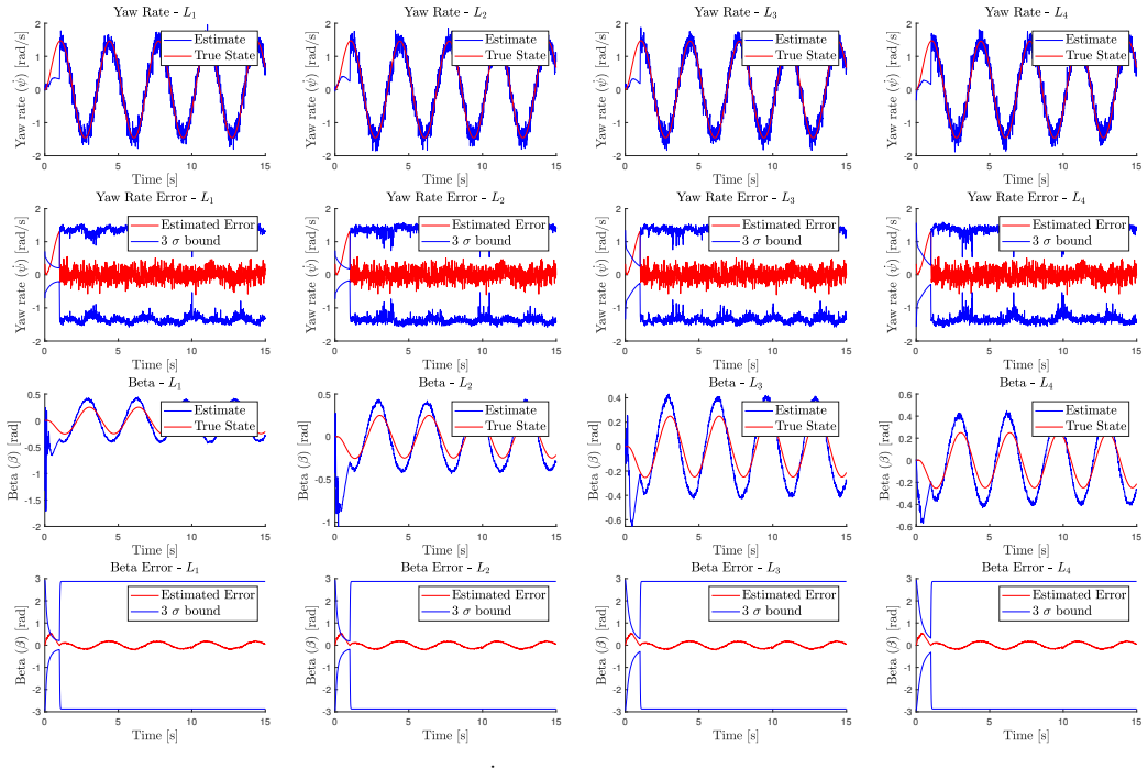
The paper's central claim is that the innovation sequence of the Kalman filter carries the information needed to identify noise covariances, and that exposing the learner to innovation-consistency statistics during training improves the downstream state estimates. An LSTM maps a sliding window of the last 100 measurements and innovations, concatenated with the previous Q and R estimates, to a prediction of the diagonal process-noise covariance Q = diag(Qa, Qb) and the measurement covariance R. The physics constraints are the time-averaged innovation autocorrelation and the normalized innovation square, two statistics that vanish or take unit mean when the filter is behaving consistently with its own covariances. Adding these terms to the loss produces lower RMSE in yaw-rate and slip-angle estimates on unseen maneuvers than training on label error alone; the paper attributes this to better identification of the noise covariances, with measurement noise identified more reliably than the process noise on the unmeasured slip-angle state.
Load-bearing premise
The method assumes that the recent measurement and innovation history carries enough information to pin down all three noise variances, including the process-noise variance for the unmeasured slip-angle state; if that information is not recoverable from yaw-rate measurements, the learned Qa will be unreliable no matter what loss is used.
Editorial extensions
If this is right
- A Kalman filter fed by a network trained with the combined loss should track yaw rate more closely on maneuvers not seen in training than a filter fed by a label-only-trained network.
- The measurement-noise variance R can be learned well enough to improve state estimation, while the process-noise variance for the unmeasured slip-angle state remains the weak point of the approach.
- Because the constraint terms are computed from a sliding window, the trained network can update Q and R in real time without running an optimization loop online.
- The loss-function ranking matters: the autocorrelation-only variant helps slip-angle estimates most, while the combined autocorrelation-plus-NIS variant helps yaw-rate estimates most.
- The benefit of physics constraints shows up mainly in the filter's output, not in raw label-prediction accuracy, so evaluating such methods requires end-to-end state-estimation metrics.
Reading between the lines
- An end-to-end extension the paper leaves implicit would differentiate through the Kalman recursion in the training loss, letting gradients reach the predicted Qa through the state estimator.
- The paper fixes the constraint weights at W2 = W3 = 0.1; a natural next step is to make them adaptive or annealed and to ablate each constraint's contribution separately.
- The Qa identifiability limit suggests that training data should include a period with direct slip-angle measurements, so the hidden process noise becomes observable at training time and the network can learn to infer it from yaw rate alone.
- Because innovation whiteness and NIS are standard filter-consistency statistics, the loss-construction recipe could transfer to other Kalman-based estimators such as integrated navigation, subject to an observability check.
Editorial analysis
A structured set of objections, weighed in public.
Referee Report
Summary. The paper proposes an LSTM-based adaptive Kalman filtering framework for a two-state bicycle model, in which a recurrent network predicts the process noise variances Qa, Qb and the measurement variance R from a moving window of yaw-rate measurements and innovations. Four loss functions are compared: label-error L1, L1 plus an innovation-autocorrelation constraint L2, L1 plus a normalized innovation square (NIS) constraint L3, and L1 plus both constraints L4. Models are trained on simulated maneuvers with random covariance labels and evaluated by label prediction error and state estimation RMSE on validation trajectories. The paper claims that adding physics-consistency terms improves state estimation through better identification of the noise covariances.
Significance. If substantiated, the result would be a useful practical step toward replacing manual covariance tuning in vehicle state estimation with a learned, real-time predictor. The paper is transparent in its Kalman filter formulation and loss definitions, and it makes a falsifiable prediction that innovation-consistency penalties improve generalization. However, the current evidence is preliminary: there are no error bars or statistical tests on the reported RMSE comparisons, no external adaptive-filtering baselines, and the paper itself concedes that the model cannot capture Qa, which is one of only three learned quantities. The significance therefore rests on a mechanism that the reported experiments do not yet establish.
major comments (4)
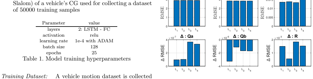
- [Section 4.2, Fig. 6] The central claim that physics constraints improve state estimation via 'better identification of process and measurement noise covariances' is not directly supported by the reported evidence. The RMSE values in Fig. 6 come from 25 random runs, but no error bars, confidence intervals, or paired statistical tests are given, so the stated differences between L2, L4, and the L1 baseline may be within run-to-run noise. Moreover, Section 4.1 (Fig. 4) shows that physics-constrained losses do not consistently improve label prediction, and Section 4.2 itself reports 'the inability of the learning model to capture the implicit information about Qa.' The paper should report mean plus/minus standard deviation or confidence intervals, apply paired significance tests between loss variants, and, ideally, show that the RMSE improvement is accompanied by lower Q/R prediction error on the same validation runs.
- [Sections 3.2-3.4 and 4.2] The proposed mechanism requires that (Qa, Qb, R) be identifiable from the innovation sequence of a single yaw-rate measurement, but this identifiability is never established. The sample autocorrelations in Eq. (13) depend on Q and R through S and P, and with one measurement channel and two process-noise channels the map from (Qa, Qb, R) to those statistics is not automatically injective; the consistency penalties in Eqs. (20)-(22) are necessary optimality conditions, not sufficient ones. The paper's own concession that Qa is 'hidden within the state estimation model' effectively concedes this problem. Please add an identifiability analysis or a simulation study showing that Qa is recoverable from the available measurements, or rephrase the causal claim to avoid attributing RMSE improvements to covariance identification.
- [Sections 4.1 and 4.2] The connection between label-prediction performance and state-estimation performance is not established. The text states that one loss variant performs best for label prediction, yet different variants are best for beta and yaw-rate RMSE, and there is no analysis of how label errors propagate to estimation errors. To support the 'better identification' mechanism, the paper should report Qa, Qb, R prediction errors on the exact validation runs used for Fig. 6, and include an oracle comparison where the filter is run with the true Q and R values, which would provide an upper bound on the achievable improvement and clarify whether the residual RMSE differences across losses are meaningful.
- [Sections 1, 4, and 5] The experimental validation is too narrow for the claims made in the abstract and conclusion. There is no comparison with existing adaptive filtering baselines, such as correlation-based covariance estimation, multiple-model adaptive estimation, or the multitask learning approach of Wu et al. (2021), and no test on real data. The evaluation only considers constant, bounded covariance values on simulated maneuvers; time-varying noise is mentioned only as future work. The paper should either add such baselines or explicitly frame the contribution as a preliminary simulation study and adjust the abstract and conclusions accordingly.
minor comments (6)
- [Section 3.2, Eq. (9)] The definition of tilde-F in Eq. (9) contains a stray comma: 'tilde-F = [F (I - WH), ]' should be a clean matrix expression.
- [Section 3.2, Eqs. (11)-(12)] The index notation is inconsistent: Eq. (11) defines C_m, while Eq. (12) uses i > 0 and refers to C_i; please harmonize the indexing.
- [Section 4.1, first paragraph] The sentence 'L∈ performs better than all other models' contains an apparent typo ('L∈'); please state which loss function is actually meant.
- [Figures 4 and 6] Both figures lack sufficient axis and legend detail: Fig. 4 does not clearly label which row is training versus validation, and Fig. 6 does not state whether the plotted RMSE values are means, medians, or individual runs, nor exactly what the black dotted baseline represents.
- [Section 3.5] Notation for the covariance matrices oscillates between Qk/Rk and Q/R, and the input vector in Eq. (18) uses hat-Q_{k-1}, hat-R_{k-1} while the text refers to 'previous timestep's Q and R'; please unify the notation.
- [Reproducibility] The paper would benefit from a data and code availability statement; the training dataset, model architecture, and hyperparameters are described, but the actual data and implementation are not released.
Circularity Check
No significant circularity: physics constraints are independent consistency conditions, and the core claim is tested on held-out trajectories.
full rationale
The derivation chain is not circular. The LSTM is trained with a supervised label loss (Eq. 19) against simulated ground-truth Qa, Qb, and R values, and the physics penalties (Eqs. 20-22) are fixed-weight consistency terms on innovation autocorrelation (Eq. 13) and normalized innovation squared (Eq. 15). These are necessary optimality conditions for a Kalman filter, not definitions of the target quantities, and the weights W2=0.1, W3=0.1 are not fitted to the evaluation data. The central state-estimation claim is assessed on validation maneuvers (Fig. 6) that are not used in training, so the RMSE comparison is an external benchmark rather than a reconstruction of the training objective. The self-referential structure in which the innovation sequence depends on the predicted Q and R is a feedback loop in the predictor-filter system, but it does not make the predicted covariances equal to their inputs by construction; the label loss anchors the predictions to independent true values. The paper's own admission in Sec. 4.2 that Qa is poorly captured (the model's inability to extract Qa hidden in the state-estimation model) describes an identifiability limitation under yaw-rate-only measurements, not a circular dependency. No load-bearing self-citation or uniqueness argument is used. Score 0.
Assumptions & free parameters
free parameters (3)
- Loss weights W2, W3 =
W2=0.1, W3=0.1
- Noise variance bound =
1e-3
- Measurement window length m =
100
assumptions (4)
- domain assumption Noise sequences are zero-mean white Gaussian with positive definite covariance matrices
- domain assumption The bicycle model with nominal cornering stiffness is an adequate filter model for the simulated plant
- standard math Innovation autocorrelation and NIS statistics are valid consistency checks for the filter
- ad hoc to paper An LSTM can approximate the mapping from measurement sequences to Q and R
Cite this review
Pith. "Pith review of Physics constrained learning of stochastic characteristics." pith.science (2026). https://pith.science/paper/3QPAIOFE
@misc{pith2026250712661,
  author       = {Pith},
  title        = {Pith review of: Physics constrained learning of stochastic characteristics},
  year         = {2026},
  howpublished = {\url{https://pith.science/paper/3QPAIOFE}},
  note         = {Machine review of arXiv:2507.12661}
}
read the original abstract
Accurate state estimation requires careful consideration of uncertainty surrounding the process and measurement models; these characteristics are usually not well-known and need an experienced designer to select the covariance matrices. An error in the selection of covariance matrices could impact the accuracy of the estimation algorithm and may sometimes cause the filter to diverge. Identifying noise characteristics has long been a challenging problem due to uncertainty surrounding noise sources and difficulties in systematic noise modeling. Most existing approaches try identifying unknown covariance matrices through an optimization algorithm involving innovation sequences. In recent years, learning approaches have been utilized to determine the stochastic characteristics of process and measurement models. We present a learning-based methodology with different loss functions to identify noise characteristics and test these approaches' performance for real-time vehicle state estimation
Figures


Figures from the paper (3 more)

Reference graph
Works this paper leans on
-
[1]
Abbeel, P., Coates, A., Montemerlo, M., Ng, A.Y., Thrun, S., et al. (2005). Discriminative training of kalman filters
work page 2005
- [2]
-
[3]
Bar-Shalom, Y., Li, X.R., and Kirubarajan, T. (2002). Estimation with Applications to Tracking and Navigation : Theory , Algorithms and Software . Wiley, 1 edition. doi:10.1002/0471221279
-
[4]
Belanger, P.R. (1972). Estimation of Noise Covariance Matrices for a Linear Time-Varying Stochastic Process . IFAC Proceedings Volumes, 5(1), 265--271. doi:10.1016/S1474-6670(17)68341-1
-
[5]
Chen, S.Y. (2012). Kalman Filter for Robot Vision : A Survey . IEEE Transactions on Industrial Electronics, 59(11), 4409--4420. doi:10.1109/TIE.2011.2162714
arXiv 2012
-
[6]
Crassidis, J.L. and Junkins, J.L. (2012). Optimal Estimation of Dynamic Systems
work page 2012
-
[7]
Giles, C.L., Lawrence, S., and Tsoi, A.C. (2001). Noisy time series prediction using recurrent neural networks and grammatical inference. Machine learning, 44, 161--183
work page 2001
-
[8]
Hilborn, C. and Lainiotis, D. (1969). Optimal Estimation in the Presence of Unknown Parameters . IEEE Transactions on Systems Science and Cybernetics, 5(1), 38--43. doi:10.1109/TSSC.1969.300242
Show all 17 references
-
[9]
HUSA, G.W. (1969). ADAPTIVE BAYES FILTERING WITH UNKNOWN PRIOR STATISTICS . Ph.D. thesis, Southern Methodist University, United States -- Texas
1969
-
[10]
Jia, X., Willard, J., Karpatne, A., Read, J.S., Zwart, J.A., Steinbach, M., and Kumar, V. (2020). Physics-guided machine learning for scientific discovery: An application in simulating lake temperature profiles. ://arxiv.org/abs/2001.11086
2020 arXiv
-
[11]
Kalman, R.E. (1960). A New Approach to Linear Filtering and Prediction Problems
1960
-
[12]
Mehra, R. (1972). Approaches to adaptive filtering. IEEE Transactions on Automatic Control, 17(5), 693--698. doi:10.1109/TAC.1972.1100100
1972
-
[13]
and Tapley, B
Myers, K. and Tapley, B. (1976). Adaptive sequential estimation with unknown noise statistics. IEEE Transactions on Automatic Control, 21(4), 520--523. doi:10.1109/TAC.1976.1101260
1976
-
[14]
(ed.) (2011)
Rajamani, R. (ed.) (2011). Vehicle dynamics and control . Springer Science & Business Media
2011
-
[15]
Salvi, A., Ala, P.S.K., Smereka, J.M., Brudnak, M., Gorsich, D., Schmid, M., and Krovi, V. (2024). Online identification of skidding modes with interactive multiple model estimation. arXiv preprint arXiv:2409.20554
2024 arXiv
-
[16]
Wu, F., Luo, H., Jia, H., Zhao, F., Xiao, Y., and Gao, X. (2021). Predicting the noise covariance with a multitask learning model for kalman filter-based gnss/ins integrated navigation. IEEE Transactions on Instrumentation and Measurement, 70, 1--13. doi:10.1109/TIM.2020.3024357
2021
-
[17]
Zhang, L., Sidoti, D., Bienkowski, A., Pattipati, K.R., Bar-Shalom , Y., and Kleinman, D.L. (2020). On the Identification of Noise Covariances and Adaptive Kalman Filtering : A New Look at a 50 Year-Old Problem . IEEE Access, 8, 59362--59388. doi:10.1109/ACCESS.2020.2982407
2020
Reviewed August 6, 2026 · model on record in the stance chip above.
Discussion (0). Sign in to comment.