REVIEW 5 major objections 5 minor 52 references
The Power of Architecture: Deep Dive into Transformer Architectures for Long-Term Time Series Forecasting
T0 review · 5 major / 5 minor · reviewed 2026-08-06 · deepseek-v4-flash
Pith's one-line read Bi-directional joint attention is the best Transformer design for long-term time series forecasting, this paper argues.
desk verdict A solid, useful taxonomy-driven comparison of Transformer architectures for LTSF; conclusions are plausible, but missing seed variance and unverified parameter matching make the evidence provisional. read the letter →
The pith
A machine-rendered reading of the paper's core claim, the machinery that carries it, and where it could break.
The reading
What carries the argument
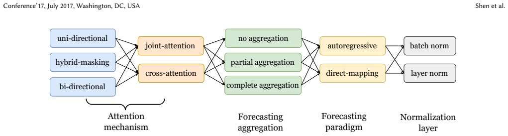
The load-bearing object is the paper's taxonomy of Transformer architectures, which separates four design dimensions: attention mechanism (bi-directional, uni-directional, or hybrid masking; joint-attention versus cross-attention), forecasting aggregation (none, partial, or complete), forecasting paradigm (direct-mapping versus autoregressive), and normalization layer (LayerNorm versus BatchNorm). The taxonomy works by holding all other design choices fixed while varying one dimension at a time, so that observed differences in MSE and MAE can be attributed to the architecture rather than to dataset-specific modeling components.
What would settle it
A controlled replication that tunes learning rate and other hyperparameters per architecture and verifies parameter counts by direct measurement could settle the claim: if a decoder-only or encoder-decoder model then matches or beats the encoder-only joint-attention model on the same datasets, the paper's central conclusion would be undermined.
Extended reading notes
Core claim
The central claim is that the architecture of a Transformer, independent of specialized time-series components, largely determines long-term forecasting quality. Concretely, the paper reports that encoder-only models using bi-directional non-causal attention with a single joint-attention module across both windows perform best; that flattening and projecting embeddings from both the look-back and forecasting windows (complete aggregation) beats projecting only forecasting tokens or each token separately; and that predicting all future values in one forward pass (direct-mapping) is far more accurate than iteratively predicting one step at a time (autoregressive). The paper further claims that BatchNorm helps on datasets with many anomalies while LayerNorm suits more stationary series. Combining these choices yields a model that the paper shows beating FEDformer, PatchTST, iTransformer, CATS, and ARMA-Attention in most cases.
Load-bearing premise
The comparisons assume that six layers in a joint-attention model give the same representational capacity as three encoder layers plus three decoder layers in a cross-attention model, and that sharing one learning rate across all architectures is fair.
Editorial extensions
If this is right
- Future Transformer designs for long-term forecasting should prefer bi-directional attention with a unified joint-attention module over separate encoder-decoder cross-attention.
- Prediction heads that flatten and project both look-back and forecasting token embeddings should be favored over per-token or forecasting-only projections.
- Direct-mapping forecasting, which emits all future values at once, should replace autoregressive generation to avoid error accumulation and training-inference mismatch.
- BatchNorm is preferable for time series with many anomalies, while LayerNorm is preferable for more stationary series with few anomalies.
- The same qualitative conclusions hold when models are trained under a variable forecasting-length setting, not just fixed-length settings.
Reading between the lines
- The taxonomy's logic could transfer to other sequence-modelling tasks: masking strategy and aggregation style likely interact with data volume, so the paper's corollary that more data shrinks the encoder-versus-decoder gap is worth testing on non-time-series data.
- A testable extension is to vary the number of layers jointly with attention type while matching parameter counts exactly; this would show whether joint-attention's advantage is architectural or partly a capacity artifact.
- Because autoregressive models here use teacher forcing, a plausible follow-up is to test whether sequence-level losses or scheduled sampling close part of the direct-mapping gap, which would separate paradigm effects from training-objective effects.
Editorial analysis
A structured set of objections, weighed in public.
Referee Report
Summary. The paper proposes a taxonomy for Transformer architectures in long-term time series forecasting, isolating four design dimensions: attention mechanism (masking strategy and joint vs. cross attention), forecasting aggregation (no/partial/complete), forecasting paradigm (direct-mapping vs. autoregressive), and normalization layer (LayerNorm vs. BatchNorm). Using controlled experiments on eight standard datasets, the authors conclude that bi-directional attention with joint-attention is most effective, that more complete forecasting aggregation improves performance, and that direct-mapping substantially outperforms autoregressive forecasting. They then build a 'combined model' from these optimal choices and report that it outperforms FEDformer, PatchTST, iTransformer, CATS, and ARMA-Attention. The manuscript includes extensive tables in the appendix, a code link, and an additional variable-forecasting-length validation.
Significance. If the comparative claims are reliable, the paper would provide practical guidance for designing Transformer-based LTSF models and a useful disentangling taxonomy that separates architectural choices from time-series-specific components. The taxonomy is well organized, the experimental coverage is broad (eight datasets, four horizons, multiple ablations), and the authors make a genuine effort to control other design choices when varying one dimension. The explicit conclusions and the availability of code are strengths. However, the central claims rest on controlled comparisons whose capacity/parameter-count equivalence is asserted rather than verified, and no uncertainty quantification is reported, so the headline conclusions are currently underdetermined.
major comments (5)
- [Section 4.1, Table 8] The statement that 'to guarantee consistent parameter counts, models with cross-attention use 3+3 layers, while models with joint-attention use 6 stacked encoder or decoder layers' is not verified anywhere in the manuscript. No parameter counts are reported. With the standard decoder block described in Appendix A, each decoder layer contains an additional cross-attention sublayer (Q, K, V, and O projections) beyond an encoder layer, so 3 encoder + 3 decoder layers will generally have more parameters than 6 encoder layers. Because Table 2 uses precisely these configurations to conclude that joint-attention is superior to cross-attention (Conclusion 1), the observed gap could be a capacity effect rather than an attention-pattern effect. Please report parameter counts for each configuration or otherwise demonstrate matched capacity, and discuss how any residual mismatch affects the conclusion.
- [Section 3.1.2 and Table 3] The three forecasting aggregation heads have very different parameter counts: 'no aggregation' uses a shared per-token projection (T × d_model to T × M parameters), 'partial aggregation' flattens T × d_model, and 'complete aggregation' flattens (L + T) × d_model before projecting to T × M. The complete-aggregation head therefore contains many more parameters than the no-aggregation head, confounding the comparison in Table 3 and the strength of Conclusion 2. The manuscript should report the parameter counts of the prediction heads (or otherwise equalize their capacity) before attributing the performance gains to the aggregation mechanism itself.
- [Tables 2–6, general experimental protocol] All results are reported as single MSE/MAE values without error bars, multiple seeds, or statistical significance tests. Several comparisons that drive the conclusions are numerically small (e.g., in Table 2, Encoder-only vs. Prefix decoder on ECL: 0.158 vs. 0.158; on Traffic: 0.385 vs. 0.383; in Table 5, Encoder-only+LN vs. +BN on ECL: 0.158 vs. 0.157). Without variance estimates it is impossible to determine whether these differences are meaningful; the paper should run at least 3–5 random seeds and report mean±std or a significance test.
- [Section 4.3, Table 6] The combined model is constructed by selecting the best-performing components on the same test benchmarks and then evaluated on those same benchmarks. This is an in-sample selection procedure, and the comparison against FEDformer, PatchTST, iTransformer, CATS, and ARMA-Attention is therefore not a fair out-of-sample test of the claimed advantage. The authors should either use a separate validation split for model selection, report a nested evaluation, or frame the combined-model results as a sanity check rather than as independent evidence for the conclusions.
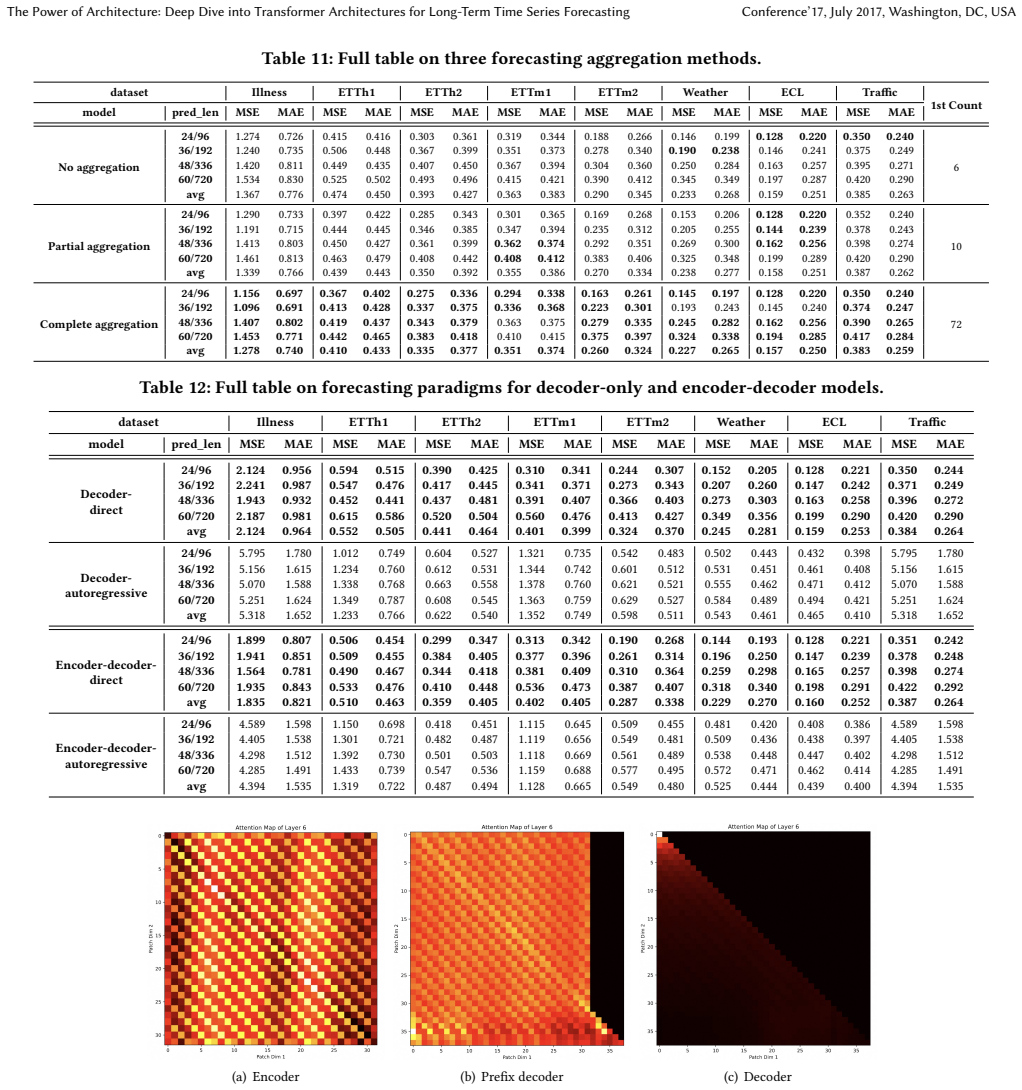
- [Section 4.2.3 and Table 4] The autoregressive models are reported to be dramatically worse than direct-mapping models (e.g., Decoder-autoregressive: 5.318 MSE on Illness vs. 2.124 for Decoder-direct; similar gaps in Table 4). The paper attributes this entirely to error accumulation and exposure bias, but all models share a single learning rate (0.001) and otherwise identical hyperparameters, and no tuning is reported for the autoregressive objective. A reasonable alternative explanation is that the autoregressive models are under-tuned (e.g., they may need different learning-rate schedules or longer training) or that the teacher-forcing procedure interacts poorly with the fixed look-back patching design. Please provide evidence that the comparison is not an artifact of hyperparameter selection, for example by tuning the autoregressive variants or by ablating teacher forcing.
minor comments (5)
- [Table 4 and Table 12] In Table 4 (and Table 12), the rows for Decoder-autoregressive and Encoder-decoder-autoregressive report identical values for Illness and Traffic (e.g., 5.318/1.652 for both models on Illness and Traffic). Different model architectures on different datasets should not produce identical MSE/MAE on all four horizons; this appears to be a copy-paste error and should be corrected.
- [Section 3.1.4] The shapes given for LayerNorm statistics are unclear: for input x ∈ R^{B×L×d}, the statement that μ(x) and σ(x) have shape R^B is only correct if normalization is over both L and d; if normalization is over features only, the shapes should be R^{B×L}. Please clarify the intended normalization axes.
- [Section 4.2.4, Table 5] The anomaly sample ratio is defined using an IQR-based threshold with 'e.g., 5%', but the exact threshold value used to produce the reported ratios (0.322, 0.127, etc.) is not stated. Please specify the threshold precisely so the result is reproducible.
- [Table 1] The table layout is difficult to parse: the column headers mix grouped model names and individual model names, and the checkmarks under 'Vanilla-Transformer' and other columns are not self-explanatory. Adding explicit row labels and separating the architecture categories with clearer grouping would improve readability.
- [Section 3.1.2] The definition of partial aggregation says 'H is in the shape of R^{T×d_model} or R^{L×d_model}', which is ambiguous about whether the look-back window, the forecasting window, or both can be used. Since the later discussion distinguishes partial (forecasting-token) from complete (both windows) aggregation, please define the two cases explicitly.
Circularity Check
Combined-model 'validation' reuses the same test benchmarks that selected each architectural choice; the component conclusions themselves are independent comparisons.
-
fitted input called prediction
[Section 4.3 (Combination of Optimal Architectures), Tables 2-6; Abstract]
"Based on the above conclusions, we construct an optimal Transformer architecture by combining the best choices, including bi-directional attention with joint-attention, complete forecasting aggregation, direct-mapping paradigm, and the BatchNorm layer. ... From the results reported in Table 6, our combined model outperforms these models in most cases. ... These results not only validate our previous conclusions but also emphasize the power and significance of Transformer architectural designs for LTSF performance."
The 'best choices' are the architectures that achieved the lowest MSE/MAE on the same test benchmarks in Tables 2-5 (e.g., bi-directional joint-attention, complete aggregation, direct-mapping, BatchNorm). The combined model is then evaluated on those same test benchmarks in Table 6, and its superiority is offered as 'validating' the conclusions. Because the component choices were selected on the basis of performance on the very same test sets, the combined model's success is an in-sample confirmation rather than an independent prediction; the validation loop reduces to observing that the empirically chosen winners win on the data that chose them.
full rationale
The paper's main architectural comparisons (attention mechanism, aggregation, paradigm, normalization) are self-contained experiments with external baselines, and none of the conclusions reduces by definition to the taxonomy categories. I found no load-bearing self-citation chain: the co-authored references (e.g., [24], [47]) are background citations, not used to justify the conclusions. The 'consistent parameter counts' claim (Section 4.1, Table 8) is an unverified assumption that could confound the joint-vs-cross attention comparison, but that is a correctness/validity concern, not circularity. The genuine circular step is the combined-model validation in Section 4.3: the optimal choices are fitted to the same test benchmarks on which the combined model is then evaluated, so the headline claim that the combined model 'reinforces' or 'validates' the conclusions is in-sample selection presented as confirmation. This is partial circularity because the individual conclusions and the external-baseline comparisons retain independent content, so the score is moderate rather than high.
Assumptions & free parameters
free parameters (3)
- Look-back window length =
512 for most datasets, 120 for Illness
- Patch length =
16 for most datasets, 6 for Illness
- Anomaly sample ratio threshold =
5%
assumptions (4)
- domain assumption Channel independence: each channel is treated as a separate univariate series.
- domain assumption Non-overlapping patching is used for all models.
- domain assumption RevIN and z-score standardization are applied to all models.
- ad hoc to paper Six layers in joint-attention models roughly match three encoder plus three decoder layers in cross-attention models in capacity.
Cite this review
Pith. "Pith review of The Power of Architecture: Deep Dive into Transformer Architectures for Long-Term Time Series Forecasting." pith.science (2026). https://pith.science/paper/I3TBZKEM
@misc{pith2026250713043,
  author       = {Pith},
  title        = {Pith review of: The Power of Architecture: Deep Dive into Transformer Architectures for Long-Term Time Series Forecasting},
  year         = {2026},
  howpublished = {\url{https://pith.science/paper/I3TBZKEM}},
  note         = {Machine review of arXiv:2507.13043}
}
read the original abstract
Transformer-based models have recently become dominant in Long-term Time Series Forecasting (LTSF), yet the variations in their architecture, such as encoder-only, encoder-decoder, and decoder-only designs, raise a crucial question: What Transformer architecture works best for LTSF tasks? However, existing models are often tightly coupled with various time-series-specific designs, making it difficult to isolate the impact of the architecture itself. To address this, we propose a novel taxonomy that disentangles these designs, enabling clearer and more unified comparisons of Transformer architectures. Our taxonomy considers key aspects such as attention mechanisms, forecasting aggregations, forecasting paradigms, and normalization layers. Through extensive experiments, we uncover several key insights: bi-directional attention with joint-attention is most effective; more complete forecasting aggregation improves performance; and the direct-mapping paradigm outperforms autoregressive approaches. Furthermore, our combined model, utilizing optimal architectural choices, consistently outperforms several existing models, reinforcing the validity of our conclusions. We hope these findings offer valuable guidance for future research on Transformer architectural designs in LTSF. Our code is available at https://github.com/HALF111/TSF_architecture.
Figures


Figures from the paper (3 more)


Reference graph
Works this paper leans on
-
[1]
Informer: Beyond efficient transformer for long sequence time-series forecasting,
H. Zhou, S. Zhang, J. Peng, S. Zhang, J. Li, H. Xiong, and W. Zhang, “Informer: Beyond efficient transformer for long sequence time-series forecasting, ” inPro- ceedings of the AAAI conference on artificial intelligence , vol. 35, no. 12, 2021, pp. 11 106–11 115
work page 2021
-
[2]
Autoformer: Decomposition transform- ers with auto-correlation for long-term series forecasting,
H. Wu, J. Xu, J. Wang, and M. Long, “Autoformer: Decomposition transform- ers with auto-correlation for long-term series forecasting, ”Advances in Neural Information Processing Systems, vol. 34, pp. 22 419–22 430, 2021
work page 2021
-
[3]
Fedformer: Frequency en- hanced decomposed transformer for long-term series forecasting,
T. Zhou, Z. Ma, Q. Wen, X. Wang, L. Sun, and R. Jin, “Fedformer: Frequency en- hanced decomposed transformer for long-term series forecasting, ” inInternational Conference on Machine Learning . PMLR, 2022, pp. 27 268–27 286
work page 2022
-
[4]
A time series is worth 64 words: Long-term forecasting with transformers,
Y. Nie, N. H. Nguyen, P. Sinthong, and J. Kalagnanam, “A time series is worth 64 words: Long-term forecasting with transformers, ” inThe Eleventh International Conference on Learning Representations , 2022
work page 2022
-
[5]
itransformer: Inverted transformers are effective for time series forecasting,
Y. Liu, T. Hu, H. Zhang, H. Wu, S. Wang, L. Ma, and M. Long, “itransformer: Inverted transformers are effective for time series forecasting, ”arXiv preprint arXiv:2310.06625, 2023
arXiv 2023
-
[6]
Timexer: Empowering transformers for time series forecasting with exogenous variables,
Y. Wang, H. Wu, J. Dong, Y. Liu, Y. Qiu, H. Zhang, J. Wang, and M. Long, “Timexer: Empowering transformers for time series forecasting with exogenous variables, ” arXiv preprint arXiv:2402.19072, 2024
arXiv 2024
-
[7]
Autoregressive moving-average attention mechanism for time series forecasting,
J. Lu, X. Han, Y. Sun, and S. Yang, “Autoregressive moving-average attention mechanism for time series forecasting, ” 2024. [Online]. Available: https://arxiv.org/abs/2410.03159
arXiv 2024
-
[8]
Pyraformer: Low-complexity pyramidal attention for long-range time series modeling and forecasting,
S. Liu, H. Yu, C. Liao, J. Li, W. Lin, A. X. Liu, and S. Dustdar, “Pyraformer: Low-complexity pyramidal attention for long-range time series modeling and forecasting, ” in International Conference on Learning Representations , 2022. [Online]. Available: https://openreview.net/forum?id=0EXmFzUn5I
work page 2022
Show all 52 references
-
[9]
Temporal fusion transformers for interpretable multi-horizon time series forecasting,
B. Lim, S. Ö. Arık, N. Loeff, and T. Pfister, “Temporal fusion transformers for interpretable multi-horizon time series forecasting, ”International Journal of Fore- casting, vol. 37, no. 4, pp. 1748–1764, 2021
2021
-
[10]
Pdformer: Propagation delay-aware dynamic long-range transformer for traffic flow prediction,
J. Jiang, C. Han, W. X. Zhao, and J. Wang, “Pdformer: Propagation delay-aware dynamic long-range transformer for traffic flow prediction, ” inProceedings of the AAAI conference on artificial intelligence , vol. 37, no. 4, 2023, pp. 4365–4373
2023
-
[11]
Basisformer: Attention-based time series forecasting with learnable and interpretable basis,
Z. Ni, H. Yu, S. Liu, J. Li, and W. Lin, “Basisformer: Attention-based time series forecasting with learnable and interpretable basis, ”Advances in Neural Informa- tion Processing Systems, vol. 36, 2024
2024
-
[12]
Samformer: Unlocking the potential of transformers in time series forecasting with sharpness-aware minimization and channel-wise attention,
R. Ilbert, A. Odonnat, V. Feofanov, A. Virmaux, G. Paolo, T. Palpanas, and I. Redko, “Samformer: Unlocking the potential of transformers in time series forecasting with sharpness-aware minimization and channel-wise attention, ” inForty-first International Conference on Machine...
-
[13]
Scaleformer: Iterative multi-scale refining transformers for time series forecasting,
A. Shabani, A. Abdi, L. Meng, and T. Sylvain, “Scaleformer: Iterative multi-scale refining transformers for time series forecasting, ”arXiv preprint arXiv:2206.04038, 2022
2022 arXiv
-
[14]
Learning to rotate: Quaternion transformer for complicated periodical time series forecasting,
W. Chen, W. Wang, B. Peng, Q. Wen, T. Zhou, and L. Sun, “Learning to rotate: Quaternion transformer for complicated periodical time series forecasting, ” in Proceedings of the 28th ACM SIGKDD conference on knowledge discovery and data mining, 2022, pp. 146–156
2022
-
[15]
Forecasting natural gas consumption in istanbul using neural networks and multivariate time series methods,
F. Demirel, S. Zaim, A. Caliskan, and P. Gokcin Ozuyar, “Forecasting natural gas consumption in istanbul using neural networks and multivariate time series methods, ”Turkish Journal of Electrical Engineering and Computer Sciences , vol. 20, pp. 695–711, 01 2012
2012
-
[16]
A review on time series forecasting techniques for building energy consumption,
C. Deb, F. Zhang, J. Yang, S. E. Lee, and K. W. Shah, “A review on time series forecasting techniques for building energy consumption, ”Renewable and Sustainable Energy Reviews , vol. 74, pp. 902–924, 2017. [Online]. Available: https://www.sciencedirect.com/science/article/pii...
2017
-
[17]
Presentation of a new hybrid approach for forecasting economic growth using artificial intelligence approaches,
M. Ahmadi, S. Ghoushchi, R. Taghizadeh, and A. Sharifi, “Presentation of a new hybrid approach for forecasting economic growth using artificial intelligence approaches, ”Neural Computing and Applications, vol. 31, p. 8661–8680, 12 2019
2019
-
[18]
Web service recommendation based on time series forecasting and collaborative filtering,
Y. Hu, Q. Peng, X. Hu, and R. Yang, “Web service recommendation based on time series forecasting and collaborative filtering, ” in 2015 IEEE International Conference on Web Services, 2015, pp. 233–240
2015
-
[19]
An econometric time series forecasting framework for web services recommendation,
V. P. Singh, M. K. Pandey, P. S. Singh, and S. Karthikeyan, “An econometric time series forecasting framework for web services recommendation, ” Procedia Computer Science , vol. 167, pp. 1615–1625, 2020, international Conference on Computational Intelligence and Data Science. ...
2020
-
[20]
Neural net time series forecasting framework for time-aware web services recommendation,
——, “Neural net time series forecasting framework for time-aware web services recommendation, ”Procedia Computer Science , vol. 171, pp. 1313–1322, 2020, third International Conference on Computing and Network Communications (CoCoNet’19). [Online]. Available: https://www.scien...
2020
-
[21]
Multivariate time series dataset for space weather data analytics,
R. Angryk, P. Martens, B. Aydin, D. Kempton, S. Mahajan, S. Basodi, A. Ah- madzadeh, X. Cai, S. Filali Boubrahimi, S. M. Hamdi, M. Schuh, and M. Georgoulis, “Multivariate time series dataset for space weather data analytics, ”Scientific Data, vol. 7, p. 227, 07 2020
2020
-
[22]
Transductive lstm for time-series prediction: An application to weather forecasting,
Z. Karevan and J. A. Suykens, “Transductive lstm for time-series prediction: An application to weather forecasting, ” Neural Networks , vol. 125, pp. 1–9,
-
[23]
Chapter 16 - copula methods for forecasting multivariate time series,
A. Patton, “Chapter 16 - copula methods for forecasting multivariate time series, ” in Handbook of Economic Forecasting , ser. Handbook of Economic Forecasting, G. Elliott and A. Timmermann, Eds. Elsevier, 2013, vol. 2, pp. 899–960. [Online]. Available: https://www.sciencedire...
2013
-
[25]
Crossformer: Transformer utilizing cross-dimension dependency for multivariate time series forecasting,
Y. Zhang and J. Yan, “Crossformer: Transformer utilizing cross-dimension dependency for multivariate time series forecasting, ” in The Eleventh International Conference on Learning Representations , 2023. [Online]. Available: https://openreview.net/forum?id=vSVLM2j9eie
2023
-
[26]
Fredformer: Fre- quency debiased transformer for time series forecasting,
X. Piao, Z. Chen, T. Murayama, Y. Matsubara, and Y. Sakurai, “Fredformer: Fre- quency debiased transformer for time series forecasting, ” inProceedings of the 30th ACM SIGKDD Conference on Knowledge Discovery and Data Mining , 2024, pp. 2400–2410
2024
-
[27]
Pathformer: Multi-scale transformers with adaptive pathways for time series forecasting,
P. Chen, Y. Zhang, Y. Cheng, Y. Shu, Y. Wang, Q. Wen, B. Yang, and C. Guo, “Pathformer: Multi-scale transformers with adaptive pathways for time series forecasting, ”arXiv preprint arXiv:2402.05956, 2024
2024 arXiv
-
[28]
Exploring the limits of transfer learning with a unified text-to-text transformer,
C. Raffel, N. Shazeer, A. Roberts, K. Lee, S. Narang, M. Matena, Y. Zhou, W. Li, and P. J. Liu, “Exploring the limits of transfer learning with a unified text-to-text transformer, ”Journal of machine learning research , vol. 21, no. 140, pp. 1–67, 2020
2020
-
[29]
What language model architecture and pretraining objective works best for zero-shot generalization?
T. Wang, A. Roberts, D. Hesslow, T. Le Scao, H. W. Chung, I. Beltagy, J. Launay, and C. Raffel, “What language model architecture and pretraining objective works best for zero-shot generalization?” in International Conference on Machine Learning. PMLR, 2022, pp. 22 964–22 984
2022
-
[30]
Decoder-only or encoder-decoder? interpreting language model as a regularized encoder-decoder,
Z. Fu, W. Lam, Q. Yu, A. M.-C. So, S. Hu, Z. Liu, and N. Collier, “Decoder-only or encoder-decoder? interpreting language model as a regularized encoder-decoder, ” arXiv preprint arXiv:2304.04052, 2023
2023 arXiv
-
[31]
Advancing transformer architecture in long-context large language models: A comprehensive survey,
Y. Huang, J. Xu, J. Lai, Z. Jiang, T. Chen, Z. Li, Y. Yao, X. Ma, L. Yang, H. Chenet al., “Advancing transformer architecture in long-context large language models: A comprehensive survey, ”arXiv preprint arXiv:2311.12351, 2023
2023 arXiv
-
[32]
A review on large language models: Architectures, applications, taxonomies, open issues and challenges,
M. A. K. Raiaan, M. S. H. Mukta, K. Fatema, N. M. Fahad, S. Sakib, M. M. J. Mim, J. Ahmad, M. E. Ali, and S. Azam, “A review on large language models: Architectures, applications, taxonomies, open issues and challenges, ”IEEE Access, 2024
2024
-
[33]
Attention is all you need,
A. Vaswani, N. Shazeer, N. Parmar, J. Uszkoreit, L. Jones, A. N. Gomez, Ł. Kaiser, and I. Polosukhin, “Attention is all you need, ”Advances in neural information processing systems, vol. 30, 2017
2017
-
[34]
A transformer-based framework for multivariate time series representation learn- ing,
G. Zerveas, S. Jayaraman, D. Patel, A. Bhamidipaty, and C. Eickhoff, “A transformer-based framework for multivariate time series representation learn- ing, ” inProceedings of the 27th ACM SIGKDD conference on knowledge discovery & data mining, 2021, pp. 2114–2124
2021
-
[35]
Tslanet: Rethinking transformers for time series representation learning,
E. Eldele, M. Ragab, Z. Chen, M. Wu, and X. Li, “Tslanet: Rethinking transformers for time series representation learning, ”arXiv preprint arXiv:2404.08472, 2024. Conference’17, July 2017, Washington, DC, USA Shen et al
2024 arXiv
-
[36]
Are self-attentions effective for time series forecasting?
D. Kim, J. Park, J. Lee, and H. Kim, “Are self-attentions effective for time series forecasting?” arXiv preprint arXiv:2405.16877, 2024
2024 arXiv
-
[37]
Transformers in time series: A survey,
Q. Wen, T. Zhou, C. Zhang, W. Chen, Z. Ma, J. Yan, and L. Sun, “Transformers in time series: A survey, ”arXiv preprint arXiv:2202.07125, 2022
2022 arXiv
-
[38]
Exploring progress in multivariate time series forecasting: Comprehensive benchmarking and heterogeneity analysis,
Z. Shao, F. Wang, Y. Xu, W. Wei, C. Yu, Z. Zhang, D. Yao, G. Jin, X. Cao, G. Cong et al., “Exploring progress in multivariate time series forecasting: Comprehensive benchmarking and heterogeneity analysis, ”arXiv preprint arXiv:2310.06119, 2023
-
[39]
Tfb: Towards comprehensive and fair benchmarking of time series forecasting methods,
X. Qiu, J. Hu, L. Zhou, X. Wu, J. Du, B. Zhang, C. Guo, A. Zhou, C. S. Jensen, Z. Sheng et al., “Tfb: Towards comprehensive and fair benchmarking of time series forecasting methods, ”arXiv preprint arXiv:2403.20150, 2024
2024 arXiv
-
[40]
Timesnet: Temporal 2d-variation modeling for general time series analysis,
H. Wu, T. Hu, Y. Liu, H. Zhou, J. Wang, and M. Long, “Timesnet: Temporal 2d-variation modeling for general time series analysis, ” in The Eleventh International Conference on Learning Representations , 2023. [Online]. Available: https://openreview.net/forum?id=ju_Uqw384Oq
2023
-
[41]
Language models are unsupervised multitask learners,
A. Radford, J. Wu, R. Child, D. Luan, D. Amodei, I. Sutskever et al., “Language models are unsupervised multitask learners, ”OpenAI blog, vol. 1, no. 8, p. 9, 2019
2019
-
[42]
Learning a trajectory using adjoint functions and teacher forcing,
N. B. Toomarian and J. Barhen, “Learning a trajectory using adjoint functions and teacher forcing, ”Neural networks, vol. 5, no. 3, pp. 473–484, 1992
1992
-
[43]
Professor forcing: A new algorithm for training recurrent networks,
A. M. Lamb, A. G. ALIAS PARTH GOYAL, Y. Zhang, S. Zhang, A. C. Courville, and Y. Bengio, “Professor forcing: A new algorithm for training recurrent networks, ” Advances in neural information processing systems , vol. 29, 2016
2016
-
[44]
Reversible instance normalization for accurate time-series forecasting against distribution shift,
T. Kim, J. Kim, Y. Tae, C. Park, J.-H. Choi, and J. Choo, “Reversible instance normalization for accurate time-series forecasting against distribution shift, ” in International Conference on Learning Representations , 2022
2022
-
[45]
Are transformers effective for time series forecasting?
A. Zeng, M. Chen, L. Zhang, and Q. Xu, “Are transformers effective for time series forecasting?” 2022
2022
-
[46]
Enhancing the locality and breaking the memory bottleneck of transformer on time series forecasting,
S. Li, X. Jin, Y. Xuan, X. Zhou, W. Chen, Y.-X. Wang, and X. Yan, “Enhancing the locality and breaking the memory bottleneck of transformer on time series forecasting, ” 2020
2020
-
[47]
Unified training of universal time series forecasting transformers,
G. Woo, C. Liu, A. Kumar, C. Xiong, S. Savarese, and D. Sahoo, “Unified training of universal time series forecasting transformers, ” in Forty-first International Conference on Machine Learning
-
[48]
One fits all: Power general time series analysis by pretrained lm,
T. Zhou, P. Niu, L. Sun, R. Jinet al., “One fits all: Power general time series analysis by pretrained lm, ”Advances in neural information processing systems , vol. 36, pp. 43 322–43 355, 2023
2023
-
[49]
A decoder-only foundation model for time- series forecasting,
A. Das, W. Kong, R. Sen, and Y. Zhou, “A decoder-only foundation model for time- series forecasting, ” inForty-first International Conference on Machine Learning
-
[50]
Timer: Generative pre-trained transformers are large time series models,
Y. Liu, H. Zhang, C. Li, X. Huang, J. Wang, and M. Long, “Timer: Generative pre-trained transformers are large time series models, ” inForty-first International Conference on Machine Learning
-
[51]
Detection of outliers using interquartile range technique from intrusion dataset,
H. Vinutha, B. Poornima, and B. Sagar, “Detection of outliers using interquartile range technique from intrusion dataset, ” in Information and decision sciences: Proceedings of the 6th international conference on ficta . Springer, 2018, pp. 511– 518. Appendix A Formulation of ...
2018
-
[2020]
Available: https://www.sciencedirect.com/science/article/pii/ S0893608020300010
[Online]. Available: https://www.sciencedirect.com/science/article/pii/ S0893608020300010
-
[2022]
Available: https://arxiv.org/abs/2202.01381
[Online]. Available: https://arxiv.org/abs/2202.01381
Reviewed August 6, 2026 · model on record in the stance chip above.
Discussion (0). Sign in to comment.