REVIEW 4 major objections 4 minor 35 references
Relation-Aware Slicing in Cross-Domain Alignment
T0 review · 4 major / 4 minor · reviewed 2026-08-06 · deepseek-v4-flash
Pith's one-line read This paper introduces relation-aware slicing distributions that replace uniform random directions in sliced Gromov-Wasserstein distances, proving semi-metric properties and square-root sample complexity while lowering GW-2 in cross-domain…
desk verdict A genuinely new slicing construction for sliced GW, but one of the three headline theoretical claims (Proposition 4.8(iii)) is wrong and needs correction before the paper can be accepted. read the letter →
The pith
A machine-rendered reading of the paper's core claim, the machinery that carries it, and where it could break.
The reading
What carries the argument
The load-bearing object is the Relation-Aware Projecting Direction (RAPD), a random unit vector obtained by taking two displacement vectors, one from each domain, normalizing them, adding and subtracting, and perturbing the normalized sum or difference by a von Mises-Fisher or power-spherical location-scale distribution. Its role is to concentrate the slicing distribution on directions where both pairwise distances shrink by the same cosine factor, so the projection does not systematically distort the relational discrepancy between the two spaces. RASD is just the marginal law of RAPD over data samples, which makes Monte Carlo sampling cheap: draw $X,X'$ from $\mu$, $Y,Y'$ from $\nu$, compute the normalized paths, toss a coin for sum or difference, then sample the perturbation.
What would settle it
Compute the ratio $\mathrm{Max\text{-}SGW}_2(\mu_n,\mu)/\mathrm{Max\text{-}SW}_2(\mu_n,\mu)$ on a compactly supported two-cluster Gaussian in $\mathbb{R}^3$ as $n$ grows; Proposition 4.9 requires this ratio to stay bounded by a universal constant, so a ratio that grows with $n$ or with cluster separation would falsify the claimed statistical rate.
Extended reading notes
Core claim
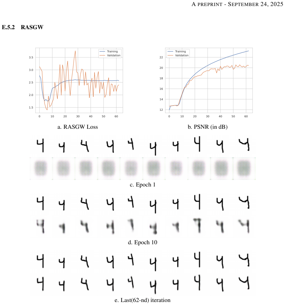
The central claim is that a data-dependent slicing distribution, rather than the uniform law on the sphere, should define sliced Gromov-Wasserstein distances. For independent pairs $(X,X')\sim \mu$ and $(Y,Y')\sim \nu$, the paper defines a Relation-Aware Projecting Direction as a location-scale perturbation around the normalized sum or difference of the displacement vectors $X-X'$ and $Y-Y'$; marginalizing over data gives the Relation-Aware Slicing Distribution (RASD). RASGW is the expectation of Gromov-Wasserstein between one-dimensional projections drawn from RASD, and IWRASGW reweights the sampled projections by an increasing function of their projected GW value. Theorem 4.7 establishes non-negativity, symmetry, identity of isometric isomorphism, and a quasi-triangle inequality; Proposition 4.8 places the new distances between SGW and Max-SGW, recovering SGW as $\kappa \to 0$ and approaching EBSGW as $L \to \infty$; Proposition 4.9 gives sample complexity $C\sqrt{(d+1)\log(n+1)/n}$. Experiments on GW-GAN and GW-autoencoder tasks support the claim that the relation-aware focus lowers the attained GW-2 distance without adding optimization overhead.
Load-bearing premise
The claimed statistical rate rests on the assumption that the worst one-dimensional projection of the Gromov-Wasserstein distance is bounded by a fixed constant times the worst one-dimensional projection of the ordinary Wasserstein distance; if that inequality holds only under extra conditions, the $O(n^{-1/2})$ guarantee is not established.
Editorial extensions
If this is right
- RASGW and IWRASGW serve as drop-in losses for GW-GANs and Gromov-Wasserstein autoencoders with the same time and memory complexity as SGW, $O(M n \log n + M d n)$ and $O(M d + M n)$, and the reported GW-2 values are lower than all tested sliced-GW baselines.
- As $\kappa \to 0$, RASGW converges to SGW; as $L \to \infty$, IWRASGW converges to EBSGW, so the new family interpolates across the existing sliced-GW spectrum.
- Both distances are semi-metrics whose zero set is the class of isometrically isomorphic spaces, and they satisfy a quasi-triangle inequality, preserving the matching semantics of Gromov-Wasserstein.
- The empirical estimator converges at the same $O(n^{-1/2})$ rate as conventional SGW under compact support, so focusing slices on informative directions costs no statistical efficiency in sample size.
- The Monte Carlo error is bounded by the standard deviation of projected GW under RASD divided by $\sqrt{M}$; varying $\kappa$ gives a direct handle on estimator variance without extra computation.
Reading between the lines
- Editorial inference: RAPD could replace the uniform sphere as a proposal for importance-sampled energy-based slicing, potentially cutting the number of slices needed for a fixed approximation accuracy; the paper does not test this.
- Editorial inference: since RAPD only requires paired displacement vectors, a relation-aware slice could be built on manifolds or graphs by substituting geodesic or shortest-path displacements for Euclidean differences; the paper proves its properties only for Euclidean projections.
- Editorial inference: because max-slicing optimizes the worst direction rather than a relation-preserving one, the hierarchy in Proposition 4.8 suggests RAPD-based alignment will beat Max-SGW more clearly in higher dimensions, where uniform directions concentrate near orthogonal to any informative direction.
Editorial analysis
A structured set of objections, weighed in public.
Referee Report
Summary. The manuscript introduces the relation-aware projecting direction (RAPD), a data-dependent distribution over the unit sphere constructed from pairwise differences of samples from the two input measures, and uses it to define two new sliced Gromov-Wasserstein distances, RASGW and IWRASGW. The main theoretical claims are semi-metricity (Theorem 4.7), a hierarchy relating RASGW/IWRASGW to SGW, Max-SGW, and EBSGW (Proposition 4.8), a sublinear sample complexity O(n^{-1/2}) (Proposition 4.9), and Monte Carlo error control (Proposition 4.10). The experimental section adapts several sliced Wasserstein methods to the GW setting and reports improved GW-2 distances in cross-domain generative tasks, as well as competitive FID/PSNR scores in autoencoder experiments.
Significance. The idea of an optimization-free, easily sampleable slicing distribution that depends on the geometry of both measures is a useful and timely contribution: it directly addresses the inefficiency of uniform slicing in high dimensions and opens a new family of sliced GW distances. The manuscript provides extensive experiments with several adapted baselines and makes code publicly available, which is a strength. However, the theoretical development is only partially sound: the claimed convergence of IWRASGW to EBSGW is incorrect as stated, and the sample complexity proof relies on an unproven inequality. These issues are load-bearing for the positioning of the proposed distances, but they appear repairable within the scope of a major revision.
major comments (4)
- [Proposition 4.8(iii) and Appendix A.2(iii)] The claim that IWRASGW converges to EBSGW as L→∞ is false for the stated definition. Definition 4.6 draws θ1,...,θL i.i.d. from σRA and uses self-normalized weights w_l = f(GW_p^p(θl♯µ, θl♯ν)). By the strong law, the limit is E_{θ∼σRA}[g(θ)f(g(θ))]/E_{θ∼σRA}[f(g(θ))], where g(θ)=GW_p^p(θ♯µ,θ♯ν). EBSGW, defined in Equation (5) of Appendix B, is E_{θ∼σ_{µ,ν}}[g(θ)] with σ_{µ,ν}(θ) ∝ f(g(θ)) relative to the uniform law on S^{d−1}, i.e., E_U[g f(g)]/E_U[f(g)]. These two quantities agree only when σRA equals the uniform law. A concrete counterexample is given by µ=(δ_{e1}+δ_{−e1})/2 and ν=(δ_{e2}+δ_{−e2})/2, for which the RAPD centers are (±e1±e2)/√2, where g(θ)=0. As κ→∞, the L→∞ limit of IWRASGW tends to 0, whereas EBSGW remains strictly positive. The proof in Appendix A.2(iii) simply asserts the convergence to EBSGW without addressing the missing proposal-density correction. This is a load-bearing claim: the abstract and Section 4.2 use it to justify IWRASGW as an energy-based slicing method.
- [Proposition 4.9 and Appendix A.3] The sample complexity proof relies on the inequality Max-SGW_p(µ_n,µ) ≤ c Max-SW_p(µ_n,µ), attributed to Zhang et al. [2024] without stating the constant or the required conditions. While this inequality is repairable for 1D projections (since GW_p ≤ 2 W_p gives Max-SGW_p ≤ 2 Max-SW_p), the proof as written is not self-contained. Additionally, the step Max-SW_p^p(µ_n,µ) ≤ diam(X) max_{x,θ} |F_{n,θ}(x)−F_θ(x)|^p is not a standard bound and appears to need a more careful treatment of the diameter and the p-th root in the final rate. The claimed O(n^{-1/2}) rate may be correct, but the derivation must be rewritten with explicit constants and assumptions.
- [Theorem 4.7] The quasi-triangle inequality is stated using objects RASGW_p^p(µ1,µ3;σκ,µ1,µ2) and RASGW_p^p(µ3,µ2;σκ,µ1,µ2) that are never defined in the main text. The notation suggests the slicing distribution is built from the pair (µ1,µ2) rather than from the measures being compared, but this is not stated explicitly. A precise definition of these quantities is needed for the statement to be meaningful.
- [Section 4, Gradient Estimation] The claim that the Monte Carlo gradient estimator is unbiased requires a reparameterization derivation for the full sampling process, including the dependence of the RAPD centers on µ_ϕ through X,X′∼µ_ϕ. The text states 'with parameterized sampling' and then writes the estimator, but does not provide the reparameterization or a proof of unbiasedness. Since this estimator is used in the GWGAN training, a rigorous statement (or a citation to a full derivation) is needed.
minor comments (4)
- [Appendix A.1] In the proof for IWRASGW, the denominator in the displayed expression is written as Σ_j GW_p^p(θj♯µ, θj♯ν) instead of Σ_j f(GW_p^p(θj♯µ, θj♯ν)); the correct denominator appears in Definition 4.6.
- [Table 2] The formatting of Table 2 is garbled: the column labels for C and O are not cleanly aligned with the reported FID, PSNR, time, and epoch entries.
- [Proposition 4.10] The statement that the variance under σRA is 'easy to control' and 'we may always observe a tighter bound than SGW' is not justified; the variance of GW_p^p under σRA could be larger than under the uniform distribution for some measures, so the comparison should be phrased conditionally.
- [Appendix D, Algorithm 5] The discussion of solving the 1D GW problem with identity or anti-identity permutations cites Vayer et al. [2019] and Beinert et al. [2023] and should clarify that this is a computational heuristic in practice, not a proven property of RASGW for arbitrary p and supports.
Circularity Check
No significant circularity; the RASGW construction and its metric/sample-complexity proofs are self-contained against external benchmarks, though Proposition 4.8(iii) is mathematically unsupported (a correctness issue, not a circular one).
full rationale
The core construction is an expectation over a new data-dependent slicing distribution and is not defined in terms of the quantities it predicts: RASGW_p^p(µ,ν;σκ) = E_{θ∼σRA}[GW_p^p(θ♯µ,θ♯ν)] uses σRA built from (µ⊗ν)^{⊗2}, and the metric and sample-complexity results are proved against external benchmarks (SGW, Max-SGW, EBSGW). No parameter is fitted to the reported GW-2 scores, and the few self-adjacent citations (e.g., Nguyen et al. 2024 for the additive constant in Remark 4.2) are not load-bearing. I therefore find no circular step. One non-circular correctness flag, located at Proposition 4.8(iii) and Appendix A.2(iii): the paper claims IWRASGW_p has L→∞ limit EBSGW_p, but Definition 4.6 weights projected distances with w_l = f(GW_p^p(θ_l♯µ,θ_l♯ν)) under samples θ_l ∼ σRA; the self-normalized limit is E_{θ∼σRA}[g(θ)f(g(θ))]/E_{θ∼σRA}[f(g(θ))], which equals EBSGW only if σRA equals the energy target σ_{µ,ν} ∝ f(g(θ)) or if the missing proposal-density correction f(g(θ))/σRA(θ) is inserted. The proof omits this correction, so the stated limit is unsupported; this is an error in the derivation chain, not a circular reduction to inputs.
Assumptions & free parameters
free parameters (3)
- concentration parameter κ =
50 (chosen via ablation, Table 3)
- energy function f =
not specified (e.g., exp)
- number of projections M or L =
500 for RASGW (ablation Table 4)
assumptions (3)
- domain assumption Max-SGW_p(μ_n,μ) ≤ c Max-SW_p(μ_n,μ) for a universal constant c
- domain assumption The slicing distribution σRA has full support on S^{d-1} or GW_p is continuous in θ
- domain assumption Measures have finite p-moments and support in Rd (or Polish), with padding for different dimensions
Cite this review
Pith. "Pith review of Relation-Aware Slicing in Cross-Domain Alignment." pith.science (2026). https://pith.science/paper/6DTVYBEI
@misc{pith2026250713194,
  author       = {Pith},
  title        = {Pith review of: Relation-Aware Slicing in Cross-Domain Alignment},
  year         = {2026},
  howpublished = {\url{https://pith.science/paper/6DTVYBEI}},
  note         = {Machine review of arXiv:2507.13194}
}
read the original abstract
The Sliced Gromov-Wasserstein (SGW) distance, aiming to relieve the computational cost of solving a non-convex quadratic program that is the Gromov-Wasserstein distance, utilizes projecting directions sampled uniformly from unit hyperspheres. This slicing mechanism incurs unnecessary computational costs due to uninformative directions, which also affects the representative power of the distance. However, finding a more appropriate distribution over the projecting directions (slicing distribution) is often an optimization problem in itself that comes with its own computational cost. In addition, with more intricate distributions, the sampling itself may be expensive. As a remedy, we propose an optimization-free slicing distribution that provides fast sampling for the Monte Carlo approximation. We do so by introducing the Relation-Aware Projecting Direction (RAPD), effectively capturing the pairwise association of each of two pairs of random vectors, each following their ambient law. This enables us to derive the Relation-Aware Slicing Distribution (RASD), a location-scale law corresponding to sampled RAPDs. Finally, we introduce the RASGW distance and its variants, e.g., IWRASGW (Importance Weighted RASGW), which overcome the shortcomings experienced by SGW. We theoretically analyze its properties and substantiate its empirical prowess using extensive experiments on various alignment tasks.
Figures


Figures from the paper (17 more)



Reference graph
Works this paper leans on
-
[2024]
Auto-encoding variational bayes
Diederik P Kingma and Max Welling. Auto-encoding variational bayes. arXiv preprint arXiv:1312.6114,
-
[1]
Near-linear time approximation algorithms for optimal transport via Sinkhorn iteration
Jason Altschuler, Jonathan Niles-Weed, and Philippe Rigollet. Near-linear time approximation algorithms for optimal transport via Sinkhorn iteration. In Advances in Neural Information Processing Systems, pages 1964–1974,
work page 1964
-
[2]
This experiment produces 4 distinct clusters in 3D space. It is also possible to use this experiment in 2D by setting the Z-axis coordinate to 0 for each cluster center, resulting in clusters lying in the XY-plane. The points are randomly assigned to one of these clusters, with the corresponding label indicating which center the point was sampled from. Th...
work page 2025
-
[5]
For example, given samples θ11,ϕ,
E Additional Experimental Details The gradient calculation of other sliced GW variants follows similarly to RASGW. For example, given samples θ11,ϕ, . . . , θHL,ϕ ∼ σRA(θ; µϕ, ν, κ), we have ∇ϕIWRASGWp p(µϕ, ν; σκ, L, H) = 1 H HX h=1 ∇ϕ LX l=1 GWp p(θhl,ϕ♯µϕ, θhl,ϕ♯ν) whl,ϕ(f ; µϕ, ν)PL j=1 whj,ϕ(f ; µϕ, ν) . E.1 Ablation Study We observe that for a given...
work page 2025
-
[7]
9 A PREPRINT - S EPTEMBER 24, 2025 Sigurdur Helgason. The radon transform on r n. In Integral Geometry and Radon Transforms, pages 1–62. Springer,
work page 2025
-
[11]
Directional Statistics in Machine Learning: a Brief Review
Suvrit Sra. Directional statistics in machine learning: a brief review. arXiv preprint arXiv:1605.00316,
-
[12]
Titouan Vayer, Rémi Flamary, Romain Tavenard, Laetitia Chapel, and Nicolas Courty. Sliced gromov-wasserstein. arXiv preprint arXiv:1905.10124,
work page Pith review arXiv 1905
-
[13]
We then discuss some related works in B
11 A PREPRINT - S EPTEMBER 24, 2025 Appendix First, we present skipped proofs in the main text in Appendix A. We then discuss some related works in B. We provide the algorithms in Appendix D. After that, we provide some additional experimental de- tails in Appendix E. Finally, we provide details on the computational infrastructure in Appendix F. For codes...
work page 2025
Show all 35 references
-
[14]
For the reverse direction, we use the same proof technique in Vayer et al. [2019]. If RASGWp(µ, ν; σk) = 0, we have R Sd−1 GWp (θ♯µ, θ♯ν) dσRA(θ; µ, ν, σk) = 12 A PREPRINT - S EPTEMBER 24, 2025
2019
-
[15]
Since σRA(θ; µ, ν, σk) is continuous due to the continuity of σk, we have GWp(θ♯µ, θ♯ν) = 0 for all θ ∈ Sd−1
Hence, we have GWp(θ♯µ, θ♯ν) = 0 for σRA(θ; µ, ν, σk)-almost surely θ ∈ Sd−1. Since σRA(θ; µ, ν, σk) is continuous due to the continuity of σk, we have GWp(θ♯µ, θ♯ν) = 0 for all θ ∈ Sd−1. Therefore, the measures are isometrically isomorphic. This follows from the proof of Theo...
2019
-
[16]
, θL ∈ Sd−1
In the reverse direction, when IWRASGWp(µ, ν; σκ, L) = 0 , it means that we havePL l=1 GWp p(θl♯µ, θl♯ν) f (GWp p(θl♯µ,θl♯ν))PL j=1 GWp p(θj ♯µ,θj ♯ν) = 0 for any θ1, . . . , θL ∈ Sd−1. Since f (GWp p(θl♯µ, θl♯ν)) > 0 for any θj, it implies that GWp p(θl♯µ, θl♯ν) = 0 for all θ...
2023
-
[17]
PL+1 i=1 aibi. First, we have: ( L+1X i=1 ai)( L+1X i=1 bi) = ( LX i=1 ai)( LX i=1 bi) + ( LX i=1 ai)bL+1 + ( LX i=1 bi)aL+1 + aL+1bL+1 ≤ L LX i=1 aibi + ( LX i=1 ai)bL+1 + ( LX i=1 bi)aL+1 + aL+1bL+1. By rearrangement inequality, we have aL+1bL+1 + aibi ≥ aL+1bi + bL+1ai for ...
2025
-
[18]
Therefore, we have σRA(θ; µ, ν, σκ) → U(Sd−1)
Therefore, we have vM F(θ; ϵ, κ) → U(Sd−1) and P S(θ; ϵ, κ) → U(Sd−1). Therefore, we have σRA(θ; µ, ν, σκ) → U(Sd−1). Now, we need to show that GWp p(θ♯µ, θ♯ν) is bounded and continuous with respective to θ. For boundedness, it is sufficient to note that the GW distance is a b...
2025
-
[19]
Further, the last inequality follows from Zhang et al. [2024]. Therefore, the proposition follows as long as we can demonstrate that E[Max-SWp(µn, µ)] ≤ C ′p (d +
2024
-
[20]
sup A∈A |µn(A) − µ(A)| # ≤ vuutE
logn/n where µn = 1 n Pn i=1 δXi with X1, . . . , Xn i.i.d ∼ µ, and C ′ > 0 is some universal constant which satisfies C = cC ′ and the outer expectation is taken with respect to X1, . . . , Xn. Using the closed-form of one-dimensional Wasserstein distance, we have: Max-SWp(µn...
2025
-
[21]
As a consequence, we obtain the conclusion of the proof
logn/n, where C ′ > 0 is some universal constant. As a consequence, we obtain the conclusion of the proof. 16 A PREPRINT - S EPTEMBER 24, 2025 A.4 Proof of Proposition 4.10 For any p ≥ 1, d ≥ 1, σκ ∈ P(Sd−1), and µ, ν∈ Pp(Rd), using Jensen’s inequality, we have: |E[ \RASGWp p(...
2025
-
[23]
1: Sample index i ∼ Categorical(α1, ..., αk) 2: Sample v ∼ U(Sd−2) 3: b ← −2κi+ √ 4κ2 i +(d−1)2 d−1 , a ← (d−1)+2κi+ √ 4κ2 i +(d−1)2 4 , m ← 4ab (1+b) − (d −
18 A PREPRINT - S EPTEMBER 24, 2025 Algorithm 1 Sampling from a mixture of vMF distributions Require: The number of vMF components k, location {ϵi}k i=1, concentration {κi}k i=1, mixture weights {αi}k i=1 , dimension d, unit vector e1 = (1, 0, ..,0). 1: Sample index i ∼ Catego...
2025
-
[24]
ln(t) − t + m ≥ ln(u) 10: h1 ← (ω, √ 1 − ω2v⊤)⊤ 11: ϵ′ ← e1 − ϵi 12: u = ϵ′ ∥ϵ′∥ 13: U = I − 2uu⊤ 14: return U h1 We proceed to introduce the power spherical distribution [De Cao and Aziz, 2020]: Definition C.2. The power spherical distribution (PS) describes a probability dis...
2020
-
[25]
lim κ→∞ Z Sd−1 g(x)f (x|ϵ, κ)dx = Z Sd−1 g(x)δϵ(x)dx
Conversely, as κ → ∞, the function f at its mode ϵ increases unboundedly, and the following conclusion holds for any uniformly bounded function g on Sd−1. lim κ→∞ Z Sd−1 g(x)f (x|ϵ, κ)dx = Z Sd−1 g(x)δϵ(x)dx. It is true since for x = ϵ, and κ → ∞we have f (ϵ|ϵ, κ) = 2κ Γ(d − 1...
2020
-
[26]
Thus, PS sampling is more efficient than vMF sampling. Moreover, parameter gradient 19 A PREPRINT - S EPTEMBER 24, 2025 Algorithm 2 Sampling from power spherical distribution Require: location parameter ϵ, concentration κ, dimension d, unit vector e1 = (1, 0, ..,0). 1: Sample ...
2025
-
[27]
Here, W2(RIµ(·, θ), RIν(·, θ)) achieves its peak when θ = x0 ∥x0∥2 and measures zero for θ orthogonal to x0
and RIµ(·, θ) = N (⟨θ, x0⟩, 1). Here, W2(RIµ(·, θ), RIν(·, θ)) achieves its peak when θ = x0 ∥x0∥2 and measures zero for θ orthogonal to x0. Randomly chosen vectors from the unit sphere tend to be nearly orthogonal in high dimensions. More precisely, the inequality P r(|⟨θ, x0...
2018
-
[28]
GW2 2(µθ, νθ) = S1(µθ, νθ) + S2(µθ, νθ), 21 A PREPRINT - S EPTEMBER 24, 2025 Algorithm 5 Relation-Aware Sliced Gromov-Wasserstein between discrete measures in an Euclidean setup Require: µ = 1 n Pn i=1 δxi ∈ P(Rd) and ν = 1 n Pn i=1 δyi ∈ P(Rd′ ), given d′ < d; number of Monte...
2025
-
[33]
Now, we aim to generate a 3D distribution for this target 2D distribution
This experiment generates 8 distinct clusters, and the points are randomly assigned to these clusters, with each cluster having its own corresponding label. Now, we aim to generate a 3D distribution for this target 2D distribution. It was performed for 10,000 iterations. x1 2....
2025
-
[34]
FC" and “Conv
activations, except for the final layer of the decoder, which uses a sigmoid activation function to ensure that the output is in the range [0, 1]. Input Image(3×64×64) Conv (3→32) + SiLU(3×64×64)→(32×32×32) Conv (32→64) + SiLU(32×32×32)→(64×16×16) Conv (64→128) + SiLU(64×16×16...
2015
-
[35]
Peak Signal-to-Noise Ratio
in using the features for the computation of FID, which are extracted from the final pooling layer of the Inception-v3 model that has been pre-trained on the ImageNet dataset [Deng et al., 2009]. Peak Signal-to-Noise Ratio. The Peak Signal-to-Noise Ratio (PSNR) is used for eva...
2009
-
[2011]
Unrolled generative adversarial networks
Luke Metz, Ben Poole, David Pfau, and Jascha Sohl-Dickstein. Unrolled generative adversarial networks. arXiv preprint arXiv:1611.02163,
-
[2013]
The power spherical distribution
Nicola De Cao and Wilker Aziz. The power spherical distribution. arXiv preprint arXiv:2006.04437,
2006 arXiv
-
[2014]
Fast algorithms for computational optimal transport and wasserstein barycenter
Wenshuo Guo, Nhat Ho, and Michael Jordan. Fast algorithms for computational optimal transport and wasserstein barycenter. In International Conference on Artificial Intelligence and Statistics, pages 2088–2097. PMLR,
-
[2016]
Augmented sliced wasserstein distances
Xiongjie Chen, Yongxin Yang, and Yunpeng Li. Augmented sliced wasserstein distances. arXiv preprint arXiv:2006.08812,
2006 arXiv
-
[2018]
Mode regularized generative adversarial networks
Tong Che, Yanran Li, Athul Paul Jacob, Yoshua Bengio, and Wenjie Li. Mode regularized generative adversarial networks. arXiv preprint arXiv:1612.02136,
-
[2019]
The Generator is designed as a four-layer Multilayer Perceptron (MLP)that processes a 256-dimensional input and produces a 2-dimensional output
proposed an architecture consisting of two primary components: the Generator (G) and the Adversary (A), which operate within an adversarial learning framework to generate and evaluate data distributions. The Generator is designed as a four-layer Multilayer Perceptron (MLP)that...
2025
-
[2020]
Imagenet: A large-scale hierarchical image database
Jia Deng, Wei Dong, Richard Socher, Li-Jia Li, Kai Li, and Li Fei-Fei. Imagenet: A large-scale hierarchical image database. In 2009 IEEE conference on computer vision and pattern recognition, pages 248–255. Ieee,
2009
-
[2021]
intro- duced the distributional sliced Wasserstein (DSW) distance. Adapting this to our context, we define the distributional sliced Gromov-Wasserstein (DSGW) distance, which is defined between two probability measuresµ ∈ Pp(Rd) and ν ∈ Pp(Rd) as: DSGWp p(µ, ν) = max ψ∈Ψ Eθ∼σψ...
2021
-
[2022]
Gromov-wasserstein averaging of kernel and distance matrices
10 A PREPRINT - S EPTEMBER 24, 2025 Gabriel Peyré, Marco Cuturi, and Justin Solomon. Gromov-wasserstein averaging of kernel and distance matrices. In International conference on machine learning, pages 2664–2672. PMLR,
2025
-
[2023]
provides belong to the cases other than the boundaries of a. While given random samples out of input distributions, it is quite challenging to identify the situation every time one calculates RASGW (or, Sliced GW), the point we try to make in the paper is that the best attaina...
2019
Reviewed August 6, 2026 · model on record in the stance chip above.
Discussion (0). Sign in to comment.