A causality inspired acceleration method for the fast temporal superposition of the finite line source solutions

Alberto Lazzarotto; Marc Basquens

REVIEW 3 major objections 8 minor 21 references

A causality inspired acceleration method for the fast temporal superposition of the finite line source solutions

T0 review · 3 major / 8 minor · reviewed 2026-08-06 · deepseek-v4-flash

Challenge this review Re-run · record.json Download PDF Read on arXiv ↗

Pith's one-line read A tolerance-based notion of causality removes the precomputation bottleneck in non-history time superposition for finite line source thermal simulations, cutting line-to-line precomputation cost by up to four orders of magnitude.

desk verdict Genuine speedup and honest benchmarks, but the a priori error guarantee is proven only for a surrogate integrand; send to review with that as the main revision point. read the letter →

arxiv 2507.18200 v1 pith:EWQ4TXCZ submitted 2025-07-24 physics.comp-ph

Marc Basquens , Alberto Lazzarotto This is my paper

classification physics.comp-ph MSC 65D3080A19 PACS 02.60.Jh44.10.+i

keywords finitelinesourcenon-historytemporalsuperpositionblocksmethodboreholeheatexchangershighlyoscillatoryintegralserrortoleranceconductionsimulationprecomputationacceleration

verification ladder T0 review T1 audit T2 compute T3 formal

The pith

A machine-rendered reading of the paper's core claim, the machinery that carries it, and where it could break.

The reading

This paper tries to remove the precomputation bottleneck in the non-history temporal superposition method for finite line source thermal simulations used in borehole heat exchanger fields. Its argument is that although the heat equation's fundamental solution is non-causal, for any chosen error tolerance one can treat a load as not yet felt at a target until it has had time to propagate; the method, called the blocks method, splits each source's load history into blocks separated by such effective causal time lags. Because each older block carries a Gaussian decay in the spectral variable $\zeta$ and only a smaller region of a line source needs to be integrated, the oscillatory integrands become tractable for adaptive Gauss–Kronrod quadrature and an asymptotic expansion, replacing the Bakhalov–Vasil'eva integrator that was slow and lacked a priori error control. The paper reports that the resulting precomputation is several orders of magnitude faster, up to about four in the line-to-line case, while keeping the maximum error below a user-supplied tolerance, which would make simulations with hundreds of boreholes and hundreds of thousands of hourly time steps practical.

What carries the argument

The load-bearing object is the block decomposition of the source function combined with the effective causality lag. A block $s_k$ is the sum of loads in a window of the past weighted by Gaussians, and it can be advanced by a recurrence that only requires the boundary loads entering and leaving the block. The lag $N_{i\to j}(\epsilon)$ is computed by solving $f(r_{ij}, N_{i\to j}\Delta t) \leq \epsilon$, where $f$ is the error of truncating the step response to a limited line region. For each block, the $\zeta$-integration nodes are fixed before simulation by running adaptive Gauss–Kronrod quadrature on a two-frequency trapezoidal surrogate of the oscillatory line factor, and the true geometry factor is then evaluated at those nodes to build the precomputed weights. The line-geometry integrals themselves are computed with a combination of Gaussian quadrature for slowly oscillating regions and an asymptotic expansion in powers of $1/\omega$ for rapidly oscillating regions, with the split point chosen by an a priori error bound; only the first, most recent block keeps the original Bakhalov–Vasil'eva treatment.

What would settle it

Run the line-to-line blocks method on a geometry outside the paper's test set, for example with lateral distance $\sigma = 2$ m, a 20-year hourly simulation, and tolerance $10^{-14}$, then compare against the direct discrete convolution of the loads with the step response evaluated in double precision. If the maximum absolute error $\|\varepsilon\|_\infty$ exceeds the requested tolerance, the claimed a priori error control does not hold in that regime.

Watch

Extended reading notes

Core claim

The paper claims that causality, understood as a tolerance-based cutoff, can be built directly into the non-history marching scheme. It defines blocks $s_k(\zeta, n\Delta t)$ of the Gaussian-smoothed load history, where block $k$ spans the time steps from $n-N_k$ to $n-N_{k-1}$ and satisfies a recurrence that lets each block be updated cheaply at every time step. For each source–target pair, the interaction only needs blocks older than the causal lag $N_{i\to j}(\epsilon)$, and each block's integrand is proportional to $e^{-\zeta^2 N_{k-1}\Delta \tilde{t}}$, suppressing oscillations in $\zeta$; for line sources the integration region over the source line is also reduced to a block-dependent interval. This makes the $\zeta$ integrals amenable to fixed Gauss–Kronrod nodes chosen once per simulation from a cheap surrogate integrand, with the true geometry factor evaluated at those nodes. The authors demonstrate numerically for point-to-point, line-to-point, and line-to-line geometries that for all tolerances tested down to $10^{-12}$ the infinity-norm error stays below the requested tolerance, at precomputation costs around four orders of magnitude lower than the original method in the line-to-line case.

Load-bearing premise

The promised per-block accuracy is guaranteed for an approximate two-frequency stand-in for the true line-geometry factor, not for the exact integrand, so a geometry whose true oscillatory structure the approximation misses could violate the stated error tolerance.

Editorial extensions

If this is right

Precomputation for a single line-to-line interaction drops from hundreds of seconds to tens of milliseconds at tolerance $10^{-12}$, reducing the cost that scales with the square of the number of boreholes.
Users set an error tolerance and the method returns a marching scheme whose maximum error is numerically shown to stay below that tolerance, instead of tuning the number of integration points blindly.
The marching structure is preserved: updating source functions costs $O(N_s)$ per time step while temperature evaluation is per interaction, keeping overall time complexity linear in the number of time steps.
Combined, these gains make non-history temporal superposition feasible for systems with hundreds of sources and hundreds of thousands of hourly steps, the regime of multi-decade borefield simulations.
At tolerances tighter than about $10^{-12}$, the number of Gaussian nodes grows rapidly, so the advertised speedup weakens for extreme precision.

Reading between the lines

Editorial extensions of the paper, not claims the author makes directly.

An implementation that wants the tolerance guarantee for arbitrary geometries should add a cheap validation step: compare the surrogate against the exact geometry factor at a few $\zeta$ values after node selection, and refine or flag when they disagree in oscillation content, for example near a line's endpoint with small lateral distance.
The same block-and-lag idea transfers to other diffusion problems with oscillatory spatial kernels, such as multi-source heat diffusion in layered or anisotropic media, whenever the kernel admits a bound that defines an influence region.
Because the blocks method is a true marching scheme, it can be used for online simulation and control where future loads are unknown; the higher per-step cost reported in the simulation phase compared with an FFT convolution is the price of that causality and matters less as the number of interacting sources grows.

Share X Bluesky LinkedIn Reddit HN

Editorial analysis

A structured set of objections, weighed in public.

Desk editor's note, referee report, and a circularity audit.

Desk Editor's Note

read the letter

Short version: this is a real methods paper with a usable speedup and one loosely supported error-control claim. It deserves a serious referee; I'd send it out, with the tolerance guarantee as the main revision point.

The genuinely new material: the block decomposition of load history with tolerance-based causal truncation, the per-block reduction of the effective line-source region, the replacement of Bakhvalov-Vasil'eva quadrature by asymptotic plus adaptive Gaussian quadrature, and the coarea-formula derivation of the line-to-line geometry factor. The core algebra checks out: block recurrence (7) is right, the change of variables to (16) is right, and the Appendix B cutoff bounds go in the conservative direction. The empirical study is honest and useful: errors are measured against direct discrete convolution, not against a fitted constant, and Figures 11-13 show errors below the requested tolerance over a good range of distances and tolerances. The precomputation speedups for line-to-line, three to four orders of magnitude, are credible and genuinely matter for borehole field simulation.

Soft spots, in rough order of size. First, the a priori error guarantee is not actually a proven guarantee for the true integrand. The zeta nodes are chosen by adaptive Gauss-Kronrod on the surrogate (29), a two-frequency trapezoidal approximation the authors themselves call rough; the true geometry factor is then evaluated at those nodes. Nothing bounds the difference between surrogate quadrature error and true quadrature error. The tests cover aligned lines with sigma-tilde >= 10 and tolerances down to 1e-12; they don't cover partially overlapping or offset line pairs, non-uniform lengths, or tighter tolerances. This is a real gap, though not one that makes the empirical speedup suspicious.

Second, the first block is excluded from the validation and still uses the unpublished [12] machinery. This is disclosed, but it means the claim "enforces a user-set tolerance" is really about blocks k>1 plus an inherited method. Third, the conclusion that combined precomputation plus simulation time is lower in the blocks method is not supported by Tables 1-2 for point-to-point and line-to-point at loose tolerances; the original is faster there. Minor, but the sentence should be fixed. Fourth, no code is shipped and the comparison baseline is the authors' own implementation of [12], which is understandable but worth noting.

None of this changes the core verdict. The method is internally consistent, the error study is extensive, and the speedup is load-bearing for multi-source, multi-decade simulations. The right outcome is peer review, not desk rejection, with a request to either prove or visibly soften the epsilon/K guarantee and to test the off-aligned geometries where the surrogate could miss oscillations.

Referee Report

3 major / 8 minor

Summary. The manuscript presents a "blocks" method to accelerate the non-history temporal superposition algorithm for finite line source (and point source) geothermal heat-transfer calculations. The load history is partitioned into time blocks; each block is associated with a spatial influence region determined by a user-set error tolerance ε, exploiting the approximate causality of heat diffusion. The resulting integrands are less oscillatory, enabling a combination of adaptive Gauss-Kronrod quadrature and asymptotic expansions for the ζ integral and for the geometry factors. The authors claim that the method enforces a user-set error tolerance, reduces precomputation cost by up to four orders of magnitude compared with the original non-history implementation in the line-to-line case, and maintains linear complexity in the number of time steps. The method is validated by comparison with direct discrete convolution for point-to-point, line-to-point, and line-to-line configurations over a range of distances and tolerances.

Significance. If correct, the claimed speedup would materially advance borefield-scale simulations by removing the precomputation bottleneck that made the non-history method impractical for hundreds of sources and hundreds of thousands of hourly steps. The manuscript has several genuine strengths: the block recurrence (7) is cleanly derived, the change of variables leading to (16) removes the endpoint singularity, the asymptotic/Gauss split (23) is sensible, and Appendix B provides concrete cutoff bounds. The error tolerance is an input rather than a fitted constant, and the empirical comparison uses an independent reference (the direct discrete convolution (32)), which strengthens the honesty of the error study. The complexity analysis and timing tables give a concrete picture of where the method helps and where it does not (the per-step simulation phase is more expensive than the original). However, the central error-control claim is not fully proven: adaptive node selection for blocks k>1 is based on a surrogate integrand, and the first block falls back on the very method the paper criticizes for lacking a priori error control.

major comments (3)

[Sections 3.3–3.4, Eqs. (28)–(30), Eq. (29)] The claimed a priori error tolerance of ε/K per block is not established for the true integrand. The Gauss-Kronrod nodes ζ_s are generated by applying the adaptive algorithm to the surrogate I_k(ζ) built from the trapezoidal two-frequency approximation (29), which the manuscript itself calls "a rough estimation." The actual precomputed quantities H_{k,s} in (30), however, use the true geometry factor v(ζ)/ζ² evaluated at those nodes. An adaptive quadrature error estimate controls only the error of the surrogate integrand; it provides no bound on the error of the true integrand at the same nodes. Since the true line-to-line factor contains a piecewise-constant α-term and β-term with up to five pieces (Eqs. (26), (45)–(46), Appendix C.2), while (29) has only two endpoint sine frequencies, a missed interior frequency band could push the true quadrature error above ε/K without the adaptive routine detecting it. The manuscript needs either a rigorous bound relating the surrogate and true integrands, a post-adaptive check on the true integrand with node refinement, or a clearly stated restriction of the guarantee to the surrogate with supporting evidence for a wider geometry class.
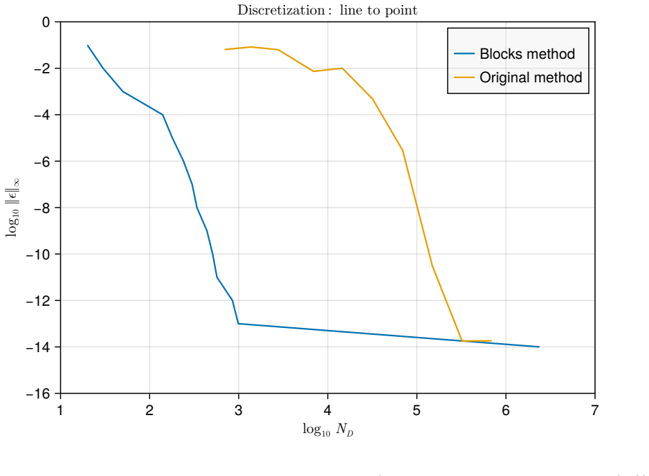
[Section 5.1, Figures 11–13] The empirical validation is too narrow to support the unrestricted claim "for all tolerances ϵ tested, ‖ε‖∞ < ϵ." All line-to-point and line-to-line tests use aligned source and target (D̃_s=D̃_t, H̃_s=H̃_t) with σ̃ ≥ 10; there are no tests with partially overlapping or offset line pairs, unequal line lengths, or tolerances below 10⁻¹². These are precisely the configurations where the surrogate approximation (29) is most likely to miss oscillation bands. Please add such tests, or qualify the error-tolerance claim accordingly; if no guarantee can be provided for these cases, the conclusions should state the applicable domain.
[Section 3.5 and Section 5, first paragraph] The method as presented does not achieve a priori error control for the first block. Section 3.5 sends k=1 back to the Bakhalov-Vasil'eva method of [12], which the Introduction (Section 2.1) identifies as lacking a priori error control; Section 5 then explicitly excludes s1 from the error study. For self-interactions and close interactions, where s1 dominates, the user-set tolerance is therefore not enforced by the new machinery. The authors should either extend error control to the first block, or state in the Abstract and Conclusions that the tolerance guarantee applies only when s1 is negligible (and quantify when this holds).

minor comments (8)

[Throughout] Standardize the transliteration of the Russian authors' names: "Bakhalov-Vasil'eva" in the Abstract, "Bakhalov-Vasil'eva" in Sections 3.5 and Appendix A, and "Bakhvalov" in reference [13] should be unified.
[Section 5.2, third bullet] The bullet heading "Line to point (Section 3.2.3)" should be "Line to line"; the discussion refers to the line-to-line integral in Section 3.2.3.
[Throughout] Typos: "compelxity" (Section 5.2), "intergrals" (Introduction), "tollerance" (Figure 1 caption), "naïve" (Introduction), and "Reisz-Fréchet" (Appendix C.2) should be corrected.
[Section 5.1] Section 5.1 uses ε both for the user tolerance and for machine precision ("ε ≃ 2 · 10⁻¹⁶"); rename the latter, e.g., ε_mach, to avoid ambiguity.
[Figures 12 and 13] Figure captions 12 and 13 state D̃=0, H̃=1500 while Section 4 uses D=0, H=150 m; clarify whether these are dimensionless with respect to r_b and define the normalization.
[Equation (36)] Equation (36) defines a synthetic load without units; state that q' is in W/m (or another unit) or that the scaling is arbitrary.
[Tables 1–3] Tables 1–3 should state whether the reported times are medians over repeated runs and specify the CPU/compiler environment; this aids reproducibility of the timing comparison.
[Section 5.1] The sentence "for all tolerances ϵ tested, ‖ε‖∞ < ϵ is kept below the specified tolerance" is redundant and should be rephrased, e.g., "in all tested cases, the maximum error stayed below the prescribed tolerance."

Circularity Check

1 steps flagged · score 2.0 of 10

Minor self-citation for the first block; the central blocks k>1 error-control claim is validated independently against direct convolution and is not circular.

self citation load bearing [Section 5.1 (Error analysis); also Section 3.5 (The first block)]
"Note that since the computation of s1 can be done with the method proposed in [12] that have already been validated there, we only assess blocks sk for k >1."

The full blocks method includes block s1, which handles close-range and self interactions. The paper's validation section explicitly excludes s1 and defers to [12], an overlapping-author manuscript under review (Lazzarotto, Basquens, and Cimmino). Section 3.5 likewise assigns s1 to the Bakhalov-Vasil'eva method 'as it was used in [12]'. Thus the completeness of the method for the full interaction range rests on an unverified self-citation rather than on evidence supplied in this paper. The central new claims for blocks k>1 are validated against the independent direct convolution (32), so this is a bounded, peripheral circular reliance rather than a collapse of the main derivation.

full rationale

The core derivation is not circular: the block decomposition (6)-(8), the block-limit selection via step-response error (9)-(10), and the per-block error budget of Section 3.4 form a genuine error decomposition, and the numerical error is measured against the independent discrete convolution (32). No parameter is fitted to the measured error, and the tolerance is an input rather than a fitted constant, so the error-control result is not a self-fulfilling fit. The main speedup claims (Tables 1-3, Figures 14-16) concern blocks k>1 and are validated against that independent reference. The only load-bearing self-citation is the handling of the first block s1, which is excluded from the validation and deferred to the authors' own prior manuscript [12] (Section 5.1 and Section 3.5). This is a genuine gap in the completeness argument, but it does not infect the validated k>1 core. Separately, the surrogate integrand (29) used to select Gauss-Kronrod nodes is explicitly called 'a rough estimation' in the paper; consequently the a priori epsilon/K guarantee is proven only for the surrogate, not rigorously for the true integrand. This is a correctness risk for untested geometries or very small tolerances, but it is not a circular step, because the final error is still compared against the independent convolution. Overall circularity is therefore limited to one minor, non-central self-citation.

Assumptions & free parameters 2 free parameters · 5 assumptions · 0 invented entities

The method introduces no new physical entities: blocks s_k and the influence region are algorithmic bookkeeping constructs, not new forces, particles, or conserved quantities. The free parameters are two hand-chosen tuning values (p = 3 for block spacing, n = 10 for asymptotic order) plus an approximate error-budget allocation in Section 3.4; none of these is fitted to the validation data. The load bound Q = max_i |q(iΔt)| is an input, not a parameter. The main unproven ingredient is the surrogate-based quadrature node placement (Eq. 29).

free parameters (2)

block spacing ratio p = 3
Section 3.1: r_{k+1} = p r_k, stated as 'an arbitrary choice, guided by the difficulty introduced by higher frequencies in the oscillatory integral. A value that yields good results is p = 3.' It affects the number of blocks and quadrature difficulty, not the accuracy guarantee itself.
asymptotic expansion truncation order n = 10
Section 5.2: 'A good balance between stability and accuracy is around n = 10'; the coefficient recurrence (19) becomes numerically unstable for larger n. This affects the accuracy and cost of the line-to-point and line-to-line precomputation.

assumptions (5)

domain assumption The heat kernel beyond the tolerance-defined influence region can be neglected, even though the heat equation is formally non-causal (Section 2.1).
The paper acknowledges the tension and adopts the posture that values below ε cannot be measured in practice. Every block truncation and influence-time computation (Eqs. 9-10) depends on this.
ad hoc to paper The surrogate (29) captures the oscillation structure of the true geometry factor well enough for adaptive quadrature node placement (Section 3.3).
The Gauss-Kronrod algorithm selects nodes from the trapezoidal surrogate, then the true v is evaluated at those nodes (Eq. 30). No error bound links the surrogate-based selection to the true integrand.
domain assumption The Bakhvalov-Vasil'eva method from [12] computes the first block s1 with adequate accuracy (Section 3.5).
[12] is an under-review preprint by two of the present authors, and Section 1 criticizes it for lacking a priori error control. The full method's error behavior for self-interactions is inherited from that unverified baseline.
standard math The coarea formula (Theorem 1, [20]) yields the piecewise-constant α and β functions used for the line-to-line factor (Appendix C.2).
A cited classical result; the paper supplies the explicit derivation of the level-set lengths and piecewise constants, so this is checkable standard mathematics.
standard math Asymptotic expansion and adaptive Gauss-Kronrod error estimates are valid for the oscillatory integrals in Section 3.2 and Appendix D.
Both are cited classical methods [13], [14], [18], [19]; the paper derives the specific coefficient recurrences (19) and the truncation bound (22) on top of them.

how reviews work

0 comments

Cite this review

Pith. "Pith review of A causality inspired acceleration method for the fast temporal superposition of the finite line source solutions." pith.science (2026). https://pith.science/paper/EWQ4TXCZ

@misc{pith2026250718200,
  author       = {Pith},
  title        = {Pith review of: A causality inspired acceleration method for the fast temporal superposition of the finite line source solutions},
  year         = {2026},
  howpublished = {\url{https://pith.science/paper/EWQ4TXCZ}},
  note         = {Machine review of arXiv:2507.18200}
}

read the original abstract

We present a novel, fast method to compute thermal interactions in solids, useful for time-dependent problems involving several sources and several time and space scales such as the ones encountered in the physics of fields of closed loop borehole heat exchangers. The new method is based on the non-history temporal superposition acceleration algorithm, but presents better performance compared to the originally proposed scheme. The main idea behind it is to leverage the propagation properties of the heat wave. Despite the basic physical solutions of heat transfer being non-causal, it is possible to establish an influence region by fixing an acceptable error tolerance. This allows to reduce the necessary integration regions in such a way that numerical integration is favored. The better behaviour of the integrand arising from this approach allows us to replace the use of Bakhalov-Vasil'eva method in favor of the asymptotic method for the computation of highly oscillatory integrals that has better properties from a computational perspective in the present application. Extensive testing is presented to evaluate the robustness of the new method and to compare its performance against the originally proposed non-history method and the convolution using the FFT algorithm for a range of error tolerances. The results show that the computational cost is highly reduced for the precomputation, which includes all the computations done before starting the time-stepping scheme. The reduction is of several orders of magnitude, depending on the specific case. This cost was the bottleneck of the original non-history implementation, and reducing it in this way makes the method suitable for simulations involving hundreds of sources and hundreds of thousands of time steps that can arise in simulations of borehole fields.

Figures

Figures reproduced from arXiv: 2507.18200 by the authors.

**Figure 2.** Visual representation of the blocks sk. The blocks partition the load history, with the first block s1 consisting of the most recent loads, and the last block sK consisting of the most distant in the past loads. The block sk is delimited by Nk, Nk−1, the number of time steps in the past from the current one. Since the blocks are fixed, as time passes, the loads flow from each block to the next, eventually accumulati… view at source ↗

**Figure 3.** provides a graphical representation of all three investigated cases along with the description of the geometric parameters that are necessary for computation [PITH_FULL_IMAGE:figures/full_fig_p009_3.png] view at source ↗

Figures from the paper (13 more)

**Figure 4.** Figure 4: Illustration of two relevant cases in the estimation of the line to point function ¯v [PITH_FULL_IMAGE:figures/full_fig_p013_4.png]

**Figure 5.** Figure 5: Summary of the integration strategy for the line to point case. The blocks structure [PITH_FULL_IMAGE:figures/full_fig_p019_5.png]

**Figure 6.** Figure 6: Integrand in equation (8), for the second block, in two cases: ( [PITH_FULL_IMAGE:figures/full_fig_p020_6.png]

**Figure 7.** Figure 7: Integrand in equation (8), for the third block, in two cases: ( [PITH_FULL_IMAGE:figures/full_fig_p021_7.png]

**Figure 8.** Figure 8: Integrand in equation (8) for the first block. [PITH_FULL_IMAGE:figures/full_fig_p021_8.png]

**Figure 9.** Figure 9: Integrand in equation (8) in two cases: ( [PITH_FULL_IMAGE:figures/full_fig_p022_9.png]

**Figure 10.** Figure 10: Integrand in equation (8) in two cases: ( [PITH_FULL_IMAGE:figures/full_fig_p023_10.png]

**Figure 11.** Figure 11: Logarithm of the ℓ ∞ norm of the error of the blocks method, for several error tolerances. The computation has been made with two different loads: (i) with a constant unit step in solid lines, and (ii) with the synthetic load (36) in dashed lines. The results show tha…

**Figure 12.** Figure 12: L2P 5.2 Computational complexity We now examine how costly it is to use the method presented in Section 3. For a single interaction, we need to compute (31). Focusing on the precomputation first, we see that one needs to compute H i→j k,s defined in (30) for each poin…

**Figure 13.** Figure 13: L2L also has complexity O(n 2 ) but can occur multiple times per integral evaluation. However, n is usually taken to be small. Since the coefficients (19) are defined recursively by multiplying increasing integers at each iteration, they become numerically unstable fo…

**Figure 14.** Figure 14: Logarithm of the error ϵ of the blocks method (with respect to the convolution (32)) against the number of discretization points ND, for both the blocks and the original method, in the point to point case. The geometric parameters used were r = 1m. The comparison betw…

**Figure 15.** Figure 15: Logarithm of the error ϵ of the blocks method (with respect to the convolution (32)) against the number of discretization points ND, for both the blocks and the original method, in the line to point case. The geometric parameters used were D = 0, H = 150m, z = 75m, σ …

**Figure 16.** Figure 16: Logarithm of the error ϵ of the blocks method (with respect to the convolution (32)) against the number of discretization points ND, for both the blocks and the original method, in the line to line case. The geometric parameters used were D˜ = 0, H˜ = 1500, D˜′ = 0, H…

Discussion (0). Sign in to comment.

Reference graph

Works this paper leans on

21 extracted references · 20 canonical work pages

[12]

A non-history dependent temporal superposition algorithm for the finite line source solution

A. Lazzarotto, M. Basquens, and M. Cimmino, “A non-history dependent temporal superpo- sition algorithm for the finite line source solution,” Under review at International Journal of Heat and Mass Transfer, 2025. [Online]. Available: https://arxiv.org/abs/2501.16027

work page Pith review arXiv 2025
[1]

Direct utilization of geothermal energy 2020 worldwide review,

J. W. Lund and A. N. Toth, “Direct utilization of geothermal energy 2020 worldwide review,” Geothermics, vol. 90, p. 101 915, 2021, issn: 0375-6505. doi: https://doi.org/10.1016/ j . geothermics . 2020 . 101915. [Online]. Available: https : / / www . sciencedirect . com / science/article/pii/S0375650520302078

work page 2020
[2]

Ashrae handbook – 2023 hvac applications,

ASHRAE, “Ashrae handbook – 2023 hvac applications,” in ASHRAE, 2023, ch. 35 : Geother- mal Energy

work page 2023
[3]

Review of analytical models for heat transfer by vertical ground heat ex- changers (ghes): A perspective of time and space scales,

M. Li and A. C. Lai, “Review of analytical models for heat transfer by vertical ground heat ex- changers (ghes): A perspective of time and space scales,”Applied Energy, vol. 151, pp. 178–191, 2015, issn: 0306-2619. doi: https://doi.org/10.1016/j.apenergy.2015.04.070. [Online]. Available: https://www.sciencedirect.com/science/article/pii/S0306261915005334

work page doi:10.1016/j.apenergy.2015.04.070 2015
[4]

An analytical method to calculate borehole fluid temperatures for time-scales from minutes to decades,

J. Claesson and S. Javed, “An analytical method to calculate borehole fluid temperatures for time-scales from minutes to decades,” English, ASHRAE Transactions., vol. 117, no. 2, pp. 279–288, 2011

work page 2011
[5]

A contribution towards the determination of g- functions using the finite line source,

M. Cimmino, M. Bernier, and F. Adams, “A contribution towards the determination of g- functions using the finite line source,” Applied Thermal Engineering, vol. 51, no. 1, pp. 401– 412, 2013, issn: 1359-4311. doi: https://doi.org/10.1016/j.applthermaleng.2012. 07.044 . [Online]. Available: https://www.sciencedirect.com/science/article/pii/ S135943111200573X

work page doi:10.1016/j.applthermaleng.2012 2013
[6]

Fast fluid and ground temperature computation for geothermal ground-loop heat exchanger systems,

D. Marcotte and P. Pasquier, “Fast fluid and ground temperature computation for geothermal ground-loop heat exchanger systems,” Geothermics, vol. 37, no. 6, pp. 651–665, 2008, issn: 0375-6505. doi: https : / / doi . org / 10 . 1016 / j . geothermics . 2008 . 08 . 003. [Online]. Available: https://www.sciencedirect.com/science/article/pii/S0375650508000552. 41

work page 2008
[7]

Characterization, testing, and optimization of load aggrega- tion methods for ground heat exchanger response-factor models,

M. S. Mitchell and J. D. Spitler, “Characterization, testing, and optimization of load aggrega- tion methods for ground heat exchanger response-factor models,” Science and Technology for the Built Environment, vol. 25, no. 8, pp. 1036–1051, 2019. doi: 10.1080/23744731.2019. 1648936

work page arXiv 2019

Show all 21 references

[8]

A multiple load aggregation algorithm for annual hourly simulations of gchp systems,

M. Bernier, P. Pinel, R. Labib, and R. Paillot, “A multiple load aggregation algorithm for annual hourly simulations of gchp systems,” HV AC&R Research, vol. 10, no. 4, pp. 471–487,
[9]

A load-aggregation method to calculate extraction temperatures of borehole heat exchangers,

J. Claesson and S. Javed, “A load-aggregation method to calculate extraction temperatures of borehole heat exchangers,” ASHRAE Transactions, vol. 118, no. 1, pp. 530–539, 2012

2012
[10]

A fast algorithm for the simulation of gchp systems,

L. Lamarche and B. Beauchamp, “A fast algorithm for the simulation of gchp systems,” ASHRAE Transactions, vol. 113, pp. 470–476, Jan. 2007

2007
[11]

A fast algorithm for the hourly simulations of ground-source heat pumps using arbitrary response factors,

L. Lamarche, “A fast algorithm for the hourly simulations of ground-source heat pumps using arbitrary response factors,” Renewable Energy, vol. 34, no. 10, pp. 2252–2258, 2009, issn: 0960-1481. doi: https://doi.org/10.1016/j.renene.2009.02.010 . [Online]. Available: https://ww...

2009 doi
[13]

Evaluation of the integrals of oscillating functions by inter- polation at nodes of gaussian quadratures,

N. Bakhvalov and L. Vasil’eva, “Evaluation of the integrals of oscillating functions by inter- polation at nodes of gaussian quadratures,” USSR Computational Mathematics and Mathe- matical Physics, vol. 8, no. 1, pp. 241–249, 1968, issn: 0041-5553. doi: https://doi.org/ 10.101...

1968
[14]

Integration with control of accuracy,

A. S. Kronrod, “Integration with control of accuracy,” Dokl. Akad. Nauk SSSR, vol. 154, pp. 283–286, 2 1964

1964
[15]

Heat conduction paradox involving second-sound propa- gation in moving media,

C. I. Christov and P. M. Jordan, “Heat conduction paradox involving second-sound propa- gation in moving media,” Phys. Rev. Lett., vol. 94, p. 154 301, 15 Apr. 2005. doi: 10.1103/ PhysRevLett . 94 . 154301. [Online]. Available: https : / / link . aps . org / doi / 10 . 1103 / ...

2005
[16]

Dispersion relations for the time-fractional cattaneo-maxwell heat equation,

A. Giusti, “Dispersion relations for the time-fractional cattaneo-maxwell heat equation,” Jour- nal of Mathematical Physics, vol. 59, no. 1, p. 013 506, Jan. 2018, issn: 0022-2488. doi: 10 . 1063 / 1 . 5001555. eprint: https : / / pubs . aip . org / aip / jmp / article - pdf /...

2018 doi
[17]

Causal heat conduction contravening the fading memory paradigm,

L. Herrera, “Causal heat conduction contravening the fading memory paradigm,” Entropy, vol. 21, no. 10, 2019, issn: 1099-4300. doi: 10.3390/e21100950. [Online]. Available: https: //www.mdpi.com/1099-4300/21/10/950. 42

2019 doi
[18]

Efficient quadrature of highly oscillatory integrals using deriva- tives,

A. Iserles and S. Norsett, “Efficient quadrature of highly oscillatory integrals using deriva- tives,” Proceedings of The Royal Society A Mathematical Physical and Engineering Sciences, vol. 461, Apr. 2005. doi: 10.1098/rspa.2004.1401

2005
[19]

Moment-free numerical integration of highly oscillatory functions,

S. Olver, “Moment-free numerical integration of highly oscillatory functions,” IMA Journal of Numerical Analysis, vol. 26, no. 2, pp. 213–227, Apr. 2006, issn: 0272-4979. doi: 10.1093/ imanum/dri040 . eprint: https://academic.oup.com/imajna/article- pdf/26/2/213/ 1971924/dri04...

2006 doi
[20]

The co-area formula for sobolev mappings,

J. Mal´ y, D. Swanson, and W. P. Ziemer, “The co-area formula for sobolev mappings,” Trans- actions of the American Mathematical Society, vol. 355, pp. 477–492, 2003. 43

2003
[2004]

[Online]

doi: 10.1080/10789669.2004.10391115 . [Online]. Available: https://doi.org/10. 1080/10789669.2004.10391115

2004

Pith tools

Reviewed August 6, 2026 · model on record in the stance chip above.

[1] [12]

A non-history dependent temporal superposition algorithm for the finite line source solution

A. Lazzarotto, M. Basquens, and M. Cimmino, “A non-history dependent temporal superpo- sition algorithm for the finite line source solution,” Under review at International Journal of Heat and Mass Transfer, 2025. [Online]. Available: https://arxiv.org/abs/2501.16027

work page Pith review arXiv 2025

[2] [1]

Direct utilization of geothermal energy 2020 worldwide review,

J. W. Lund and A. N. Toth, “Direct utilization of geothermal energy 2020 worldwide review,” Geothermics, vol. 90, p. 101 915, 2021, issn: 0375-6505. doi: https://doi.org/10.1016/ j . geothermics . 2020 . 101915. [Online]. Available: https : / / www . sciencedirect . com / science/article/pii/S0375650520302078

work page 2020

[3] [2]

Ashrae handbook – 2023 hvac applications,

ASHRAE, “Ashrae handbook – 2023 hvac applications,” in ASHRAE, 2023, ch. 35 : Geother- mal Energy

work page 2023

[4] [3]

Review of analytical models for heat transfer by vertical ground heat ex- changers (ghes): A perspective of time and space scales,

M. Li and A. C. Lai, “Review of analytical models for heat transfer by vertical ground heat ex- changers (ghes): A perspective of time and space scales,”Applied Energy, vol. 151, pp. 178–191, 2015, issn: 0306-2619. doi: https://doi.org/10.1016/j.apenergy.2015.04.070. [Online]. Available: https://www.sciencedirect.com/science/article/pii/S0306261915005334

work page doi:10.1016/j.apenergy.2015.04.070 2015

[5] [4]

An analytical method to calculate borehole fluid temperatures for time-scales from minutes to decades,

J. Claesson and S. Javed, “An analytical method to calculate borehole fluid temperatures for time-scales from minutes to decades,” English, ASHRAE Transactions., vol. 117, no. 2, pp. 279–288, 2011

work page 2011

[6] [5]

A contribution towards the determination of g- functions using the finite line source,

M. Cimmino, M. Bernier, and F. Adams, “A contribution towards the determination of g- functions using the finite line source,” Applied Thermal Engineering, vol. 51, no. 1, pp. 401– 412, 2013, issn: 1359-4311. doi: https://doi.org/10.1016/j.applthermaleng.2012. 07.044 . [Online]. Available: https://www.sciencedirect.com/science/article/pii/ S135943111200573X

work page doi:10.1016/j.applthermaleng.2012 2013

[7] [6]

Fast fluid and ground temperature computation for geothermal ground-loop heat exchanger systems,

D. Marcotte and P. Pasquier, “Fast fluid and ground temperature computation for geothermal ground-loop heat exchanger systems,” Geothermics, vol. 37, no. 6, pp. 651–665, 2008, issn: 0375-6505. doi: https : / / doi . org / 10 . 1016 / j . geothermics . 2008 . 08 . 003. [Online]. Available: https://www.sciencedirect.com/science/article/pii/S0375650508000552. 41

work page 2008

[8] [7]

Characterization, testing, and optimization of load aggrega- tion methods for ground heat exchanger response-factor models,

M. S. Mitchell and J. D. Spitler, “Characterization, testing, and optimization of load aggrega- tion methods for ground heat exchanger response-factor models,” Science and Technology for the Built Environment, vol. 25, no. 8, pp. 1036–1051, 2019. doi: 10.1080/23744731.2019. 1648936

work page arXiv 2019