REVIEW 4 major objections 6 minor 21 references
Self-Supervised Coarsening of Unstructured Grid with Automatic Differentiation
T0 review · 4 major / 6 minor · reviewed 2026-08-15 · deepseek-v4-flash
Pith's one-line read This paper claims that an unstructured computational grid can be coarsened up to tenfold—in one test from 90,000 to 1,000 points—while preserving the simulated pressure history at designated measurement points, by treating the…
desk verdict Genuinely novel differentiable coarsening pipeline with public code, but the headline accuracy claims are mostly in-sample fits; the extrapolation evidence needs to be quantified before the coarsening claim stands. read the letter →
The pith
A machine-rendered reading of the paper's core claim, the machinery that carries it, and where it could break.
The reading
What carries the argument
The mechanism is the combination of a differentiable Voronoi tessellation with a graph-based finite-volume solver. Cell areas and edge lengths are computed analytically from Delaunay triangle circumcenters and the shoelace formula, making them tensors that carry gradients, while the solver is implemented as message passing on the Voronoi graph with edge weights $w_{ij}=-A_{ij}$ and the explicit Euler update $p^{k+1}=p^k+\tau(f^k-D^{-1}Ap^k)$. This construction lets the RMSE loss at measurement points back-propagate into the coarse site coordinates, which is what turns grid coarsening into an optimization problem rather than a one-shot averaging.
What would settle it
Run any optimized coarse grid from the paper, with point locations frozen, on a scenario the optimizer never saw—a moved well, a different source rate, a changed permeability field, or a holdout measurement point—and compute the RMSE against the fine-grid simulation. If the error at holdout locations or under changed forcing is much larger than the training-time RMSE, the coarsening is fitting the training observations rather than discovering a transferable reduced model.
Extended reading notes
Core claim
The central claim is that a coarse grid can be learned rather than hand-constructed: instead of only averaging permeabilities over k-means clusters, the coarse point locations themselves are optimized to minimize the mismatch between coarse and fine simulations at points of interest. The paper shows that all geometric inputs to the finite-volume scheme—Voronoi edge lengths, cell areas, distances between sites, and harmonic-averaged permeability—are smooth functions of the site coordinates, so the simulation becomes end-to-end differentiable and the RMSE loss can drive the point positions. Reported results include a 10x reduction in grid size while preserving the modelled variable dynamics at sink points, a 90,000-to-1,000-point coarsening whose optimized grid reaches RMSE 0.042 versus 0.057 for the non-optimized reduced grid, and a wave-equation case with two sink points showing the approach is not limited to parabolic problems. The paper also states that the pipeline applies to an arbitrary evolutionary PDE, provided a finite-volume explicit solver for it can be represented over a cloud of cell centres.
Load-bearing premise
The premise on which the whole result rests is that a coarse grid tuned to match the fine-grid pressure history at a few fixed measurement points will also match the fine-grid solution later in time and at other locations; if it does not, the reported RMSE values describe curve fitting to the training points, not genuine coarsening.
Editorial extensions
If this is right
- A grid reduced by 10x can reproduce fine-grid dynamics at the measurement points, so reservoir proxy models obtained this way would run dramatically faster—about 34x in the demonstrated 90,000-to-1,000-point case.
- Because the pipeline works for both a parabolic flow equation and the hyperbolic wave equation, the same optimization loop can be reused for other explicit finite-volume PDE solvers without changing the coarsening logic.
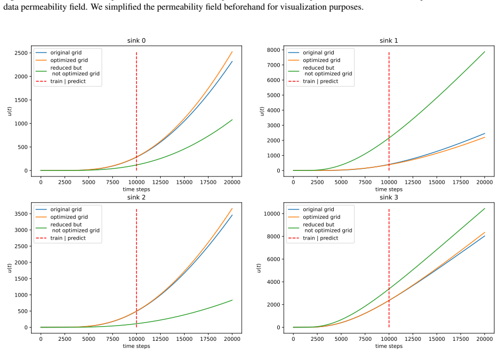
- The optimized coarse grid extends beyond the training window: in the petroleum example, the grid trained on the first 10,000 steps continues to follow the fine-grid solution for another 20,000 steps, as the authors demonstrate qualitatively.
- No training data from other mesh-adaptation methods is required, and no Hessian or adjoint error indicators are needed; the loss is the direct mismatch of the modelled variable at points of interest.
Reading between the lines
- One extension the paper leaves implicit is multi-scenario training: including several source/sink configurations and several permeability fields in the loss would produce a coarsened grid that is a general reduced-order model rather than a proxy tuned to one well pattern.
- Because point coordinates move continuously, degeneracies such as vanishing cell areas or near-crossing Voronoi edges are a natural risk; a geometric regularizer on cell area would be a direct robustness test.
- The same gradient signal could drive refinement as well as coarsening: locally large loss gradients identify regions where the coarse grid is failing, suggesting an adaptive mesh strategy that adds points where the dynamics matter.
- A natural benchmark would compare the learned coarse grid against other point-placement strategies with the same number of points, isolating how much of the gain comes from the loss-driven relocation.
Signed reviews
Editorial analysis
A structured set of objections, weighed in public.
Referee Report
Summary. The manuscript presents a differentiable-physics pipeline for coarsening unstructured finite-volume grids. Given an original point cloud and a discrete permeability field, the method forms a coarse grid via k-means clustering and then optimizes the coarse site locations by gradient descent to minimize the mean squared error between the pressure time series produced at measurement points (sinks) by the coarse and fine finite-volume simulations. The simulation is made differentiable through a differentiable Voronoi tessellation and an explicit-Euler message-passing implementation. The authors demonstrate the approach on a linear parabolic equation (slightly compressible fluid flow), with reduction ratios down to 90,000-to-1,000 points, and on the wave equation, reporting a 34x speedup and RMSE improvements over k-means plus averaging. Section 4.4 and Appendix D include a train/predict split with a longer prediction interval, presented visually in Fig. 11.
Significance. If the predictive-quality claim held, the method would be a useful contribution: it offers a principled, gradient-based route to task-oriented grid coarsening for explicit finite-volume solvers on Voronoi meshes, and the release of the code supports reproducibility. The paper also deserves credit for explicitly acknowledging the explicit-Euler stability restriction (Appendix C) and for testing on a second PDE family (the wave equation). However, the current evidence primarily demonstrates in-sample curve fitting of the coarse-model response at the measurement points, and the abstract's generality claim is stronger than the demonstrated scope. With additional holdout and forcing-perturbation experiments, the contribution could be solid; as it stands, the main claims are not fully established.
major comments (4)
- [§3.4 / Eq. (12) and §4.5 / Figs. 5–6] The optimization objective in Eq. (12) is exactly the RMSE between the coarse and fine pressure series at the measurement points that is then reported as the quality metric in Figs. 5–6 and Section 4.5 (RMSE 0.042). These numbers therefore measure training-set fit, not predictive accuracy. Appendix D attempts a train/predict split (m=10,000 training steps, m=20,000 prediction) but reports no holdout RMSE or other error metric, only visual overlap in Fig. 11, and the prediction period uses the same forcing scenario and the same measurement locations as the training period. To support the central claim that the coarse grid 'preserves the modeled variable dynamics in the points of interest' (Abstract), the authors should report quantitative holdout errors (e.g., RMSE on the withheld interval, at unconstrained locations, and under changed well configurations or boundary conditions) with repeated seeds and error bars.
- [Abstract and Conclusion] The abstract's claim that the approach 'can be applied to an arbitrary system described by evolutionary partial differential equations' is not supported by the experiments and is contradicted by the conclusion, which restricts the method to 'any finite volume, two-dimensional explicit solver' with operators representable via Voronoi tessellation. Only one parabolic and one scalar hyperbolic equation are demonstrated, and the explicit-Euler discretization is a stated limitation (Section 3.1 and Appendix C). The authors should revise the general claim to match the demonstrated scope, or add evidence for nonlinearities, systems of equations, and implicit or other discretizations.
- [§4.5 and Appendix C] The 34x speedup claim is based on running the coarse grid with the same number of time steps as the fine grid, but the explicit stability condition (Eq. 19) depends on the smallest cell area, which the optimizer can alter during training. The paper does not report whether the optimized coarse grids remain stable with the stated time step, nor does it give the minimum cell area or any verification of the CFL condition after optimization; if a smaller τ is needed, the speedup would be reduced. In addition, the speedup omits the optimization cost: for the 90,000→1,000 case, one optimization epoch takes 0.9 min (Table 3), so 60 epochs ≈ 54 min, which exceeds the 17-min fine-grid simulation (Table 2). The manuscript should state the wall-clock amortization conditions under which the method is competitive for repeated simulations.
- [§4.2 and §4.5] No error bars or repeated-run statistics are reported for any of the RMSE results, even though the pipeline is stochastic (random k-means initialization and Adam optimization). The claimed improvement from 0.057 to 0.042 in Section 4.5 appears to come from a single run; without seeds, repetitions, or confidence intervals, the reader cannot assess the robustness of the improvement. This is load-bearing because the headline quantitative claims are single-run numbers.
minor comments (6)
- [Eq. (3)] Equation (3) appears to contain a typo: the factor '2KjKj' should likely be '2KiKj' (the harmonic mean of the two adjacent-cell permeabilities). Please verify the formula and correct it.
- [Conclusion] The conclusion states 'we reduced the problem size 10 times whilst preserving preserved the quality' — the duplicated word 'preserved' should be removed, and the stated factor '10 times' conflicts with the 90,000→1,000 experiment (90x reduction) and the abstract's 'up to 10 times'. Please clarify the actual maximum reduction factor.
- [§4.4 / Appendix D] The text says 'Appedix D' (typo). More importantly, the offline video links and visual overlap in Fig. 11 are not sufficient for quantitative evaluation; the authors should provide numeric errors for the holdout period in Appendix D and for the wave equation in Appendix B.
- [Appendix B] The wave-equation experiment is described without specifying the number of optimization epochs, learning rate, or random seed, and Fig. 9 shows no error metric. Please add these details for reproducibility.
- [§4.1] The sentence 'we use sink point/measurement point interchangeably' is misleading, since a sink is a physical well with a source term (Eq. 13) while a measurement point may be a passive observation location. Please clarify the distinction.
- [Conclusion] The sentence 'Our method is focused on a specific method for solving PDE but not specific types of PDEs' is confusing; it should be rephrased as 'focused on a specific discretization (finite volumes)' rather than 'a specific method for solving PDE'.
Circularity Check
The headline RMSE of 0.042 is the optimized training loss itself, so the in-sample 'preserved dynamics' claim is a fit; only qualitative holdout curves in Appendix D provide independent evidence.
-
fitted input called prediction
[Section 3.4, Eq. (12); Section 4.5, scalability experiment]
"Finally, we formulate the following optimization problem: min S∗ MSE (ps(S), ps(S∗)) (12) ... after just 60 epochs, our model achieved an RMSE of approximately 0.042, signifying a notable improvement over the baseline k-means + average pooling result of 0.057."
The coarse-grid coordinates S∗ are optimized to minimize exactly the MSE between coarse and fine pressure at the sink/measurement points. The reported RMSE≈0.042 is therefore the final value of the training objective, not an independent measure of preserved dynamics. The abstract's claim of 'preserving the modeled variable dynamics in the points of interest' restates the loss being minimized: any optimization run that lowers this loss will, by construction, lower the reported RMSE on the same time interval and at the same points. The only genuinely out-of-sample evidence is the qualitative train/predict split in Appendix D, which reports no holdout error metric and keeps the same measurement locations, so the headline numerical improvements remain fits rather than predictions.
full rationale
The paper's main numerical evidence is the RMSE between the coarse-grid and fine-grid pressure time series at the measurement/sink points. That is precisely the objective minimized in Eq. (12), so reporting RMSE≈0.042 after 60 epochs is reporting the final value of the training loss, not an independent evaluation; the abstract's 'preserving the modeled variable dynamics in the points of interest' therefore holds by construction on the training interval. The paper does attempt a genuine out-of-sample check in Appendix D (train on 10,000 steps, then simulate to 20,000), which prevents a full 6+ circularity verdict. However, that check is only qualitative: no holdout RMSE, no error bars, no changed forcing scenario, and the same sink locations are used for fitting and testing. The self-citation to the prior differentiable Voronoi tessellation work (Shumilin et al., 2024) is not load-bearing circularity: the paper supplies the analytical formulas and code, and the tessellation is a component rather than a result derived from the claim being tested. Overall, there is one fitted-metric-as-evidence step, partially redeemed by a qualitative extrapolation experiment; the numerical discretization itself is standard and not circular.
Assumptions & free parameters
free parameters (3)
- Target coarse grid size n / reduction degree r =
r = 0.75, 0.5, 0.25; also N=90000 to n=1000, 500, 100
- Optimization schedule: epochs and learning rate =
20 to 60 epochs, Adam learning rate 1e-3
- k-means initialization state =
unspecified, no seed reported
assumptions (5)
- domain assumption The fine-grid finite-volume solution is an acceptable ground truth for the coarse grid to match.
- domain assumption The differentiable Voronoi tessellation remains valid and differentiable after every site movement, including topology changes, boundary clipping, and non-degenerate Delaunay configurations.
- domain assumption A coarse grid fitted on a finite training time window generalizes to later times and to the modeled variable at the chosen measurement points.
- domain assumption The two-point flux approximation with per-cell permeabilities, Eq. (3), remains accurate for the heterogeneous fields after aggressive coarsening.
- standard math The explicit Euler time step satisfies the stability bound stated in Appendix C.
Cite this review
Pith. "Pith review of Self-Supervised Coarsening of Unstructured Grid with Automatic Differentiation." pith.science (2026). https://pith.science/paper/PGY644BU
@misc{pith2026250718297,
  author       = {Pith},
  title        = {Pith review of: Self-Supervised Coarsening of Unstructured Grid with Automatic Differentiation},
  year         = {2026},
  howpublished = {\url{https://pith.science/paper/PGY644BU}},
  note         = {Machine review of arXiv:2507.18297}
}
read the original abstract
Due to the high computational load of modern numerical simulation, there is a demand for approaches that would reduce the size of discrete problems while keeping the accuracy reasonable. In this work, we present an original algorithm to coarsen an unstructured grid based on the concepts of differentiable physics. We achieve this by employing k-means clustering, autodifferentiation and stochastic minimization algorithms. We demonstrate performance of the designed algorithm on two PDEs: a linear parabolic equation which governs slightly compressible fluid flow in porous media and the wave equation. Our results show that in the considered scenarios, we reduced the number of grid points up to 10 times while preserving the modeled variable dynamics in the points of interest. The proposed approach can be applied to the simulation of an arbitrary system described by evolutionary partial differential equations.
Figures


Figures from the paper (7 more)


Reference graph
Works this paper leans on
-
[1]
write newline
" write newline "" before.all 'output.state := FUNCTION n.dashify 't := "" t empty not t #1 #1 substring "-" = t #1 #2 substring "--" = not "--" * t #2 global.max substring 't := t #1 #1 substring "-" = "-" * t #2 global.max substring 't := while if t #1 #1 substring * t #2 global.max substring 't := if while FUNCTION format.date year duplicate empty "emp...
-
[2]
VORONOI DIAGRAMS AND DELAUNAY TRIANGULATIONS
Aurenhammer, F., Klein, R., and Lee, D.-T. VORONOI DIAGRAMS AND DELAUNAY TRIANGULATIONS. World Scientific Publishing Co. Pte. Ltd., 1st edition, 2013
work page 2013
-
[3]
Braden, B. The surveyor's area formula. The College Mathematics Journal, 17 0 (4): 0 326--337, 1986
work page 1986
-
[4]
Reservoir Simulation: Mathematical Techniques in Oil Recovery
Chen, Z. Reservoir Simulation: Mathematical Techniques in Oil Recovery. Society for Industrial and Applied Mathematics, January 2007. ISBN 9780898717075. doi:10.1137/1.9780898717075. URL http://dx.doi.org/10.1137/1.9780898717075
-
[5]
Differentiable graph-structured models for inverse design of lattice materials
Dold, D. and van Egmond, D. A. Differentiable graph-structured models for inverse design of lattice materials. arXiv preprint arXiv:2304.05422, 2023
work page Pith review arXiv 2023
-
[6]
Finite volume methods, pp.\ 713–1018
Eymard, R., Gallouët, T., and Herbin, R. Finite volume methods, pp.\ 713–1018. Elsevier, 2000. doi:10.1016/s1570-8659(00)07005-8. URL http://dx.doi.org/10.1016/s1570-8659(00)07005-8
-
[7]
and Lenssen, J
Fey, M. and Lenssen, J. E. Fast graph representation learning with PyTorch Geometric . In ICLR Workshop on Representation Learning on Graphs and Manifolds, 2019
2019
-
[8]
Fidkowski, K. J. and Chen, G. Metric-based, goal-oriented mesh adaptation using machine learning. Journal of Computational Physics, 426: 0 109957, 2021. ISSN 0021-9991. doi:https://doi.org/10.1016/j.jcp.2020.109957. URL https://www.sciencedirect.com/science/article/pii/S0021999120307312
arXiv 2021
Show all 21 references
-
[9]
and Hesthaven, J
Guo, M. and Hesthaven, J. S. Data-driven reduced order modeling for time-dependent problems. Computer Methods in Applied Mechanics and Engineering, 345: 0 75–99, March 2019. ISSN 0045-7825. doi:10.1016/j.cma.2018.10.029. URL http://dx.doi.org/10.1016/j.cma.2018.10.029
2019 doi
-
[10]
Learning to control pdes with differentiable physics
Holl, P., Koltun, V., and Thuerey, N. Learning to control pdes with differentiable physics. arXiv preprint arXiv:2001.07457, 2020
2001 arXiv
-
[11]
F., and Bergman, L
Kerschen, G., Golinval, J.-c., Vakakis, A. F., and Bergman, L. A. The method of proper orthogonal decomposition for dynamical characterization and order reduction of mechanical systems: an overview. Nonlinear dynamics, 41: 0 147--169, 2005
2005
-
[12]
N., Brunton, S
Kutz, J. N., Brunton, S. L., Brunton, B. W., and Proctor, J. L. Dynamic Mode Decomposition: Data-Driven Modeling of Complex Systems. Society for Industrial and Applied Mathematics, November 2016. ISBN 9781611974508. doi:10.1137/1.9781611974508
2016 doi
-
[13]
Numerical analysis of a two-level preconditioner for the diffusion equation with an anisotropic diffusion tensor
Kuznetsov, Y., Boiarkine, O., Kapyrin, I., and Yavich, N. Numerical analysis of a two-level preconditioner for the diffusion equation with an anisotropic diffusion tensor. Russian Journal of Numerical Analysis and Mathematical Modelling, 22 0 (4): 0 377--391, 2007. doi:doi:10....
2007 doi
-
[14]
and Lin, M
Liang, J. and Lin, M. C. Differentiable physics simulation. In ICLR 2020 Workshop on Integration of Deep Neural Models and Differential Equations, 2020
2020
-
[15]
The art of differentiating computer programs : an introduction to algorithmic differentiation
Naumann, U. The art of differentiating computer programs : an introduction to algorithmic differentiation. SIAM, 1st edition, 2012. ISBN ISBN 978-1-611972-06-1
2012
-
[16]
A., Loseille, A., Krakos, J., Michal, T
Park, M. A., Loseille, A., Krakos, J., Michal, T. R., and Alonso, J. J. Unstructured grid adaptation: status, potential impacts, and recommended investments towards cfd 2030. In 46th AIAA fluid dynamics conference, pp.\ 3323, 2016
2016
-
[17]
Automatic differentiation in pytorch
Paszke, A., Gross, S., Chintala, S., Chanan, G., Yang, E., DeVito, Z., Lin, Z., Desmaison, A., Antiga, L., and Lerer, A. Automatic differentiation in pytorch. 2017
2017
-
[18]
and Hesketh, T
Qi, D. and Hesketh, T. An analysis of upscaling techniques for reservoir simulation. Petroleum Science and Technology, 23 0 (7–8): 0 827–842, July 2005. ISSN 1532-2459. doi:10.1081/lft-200033132
2005 doi
-
[19]
Rowley, C. W. Model reduction for fluids, using balanced proper orthogonal decomposition. International Journal of Bifurcation and Chaos, 15 0 (03): 0 997--1013, 2005
2005
-
[20]
and Cubuk, E
Schoenholz, S. and Cubuk, E. D. Jax md: a framework for differentiable physics. Advances in Neural Information Processing Systems, 33: 0 11428--11441, 2020
2020
-
[21]
A method for auto-differentiation of the voronoi tessellation, 2024
Shumilin, S., Ryabov, A., Barannikov, S., Burnaev, E., and Vanovskii, V. A method for auto-differentiation of the voronoi tessellation, 2024
2024
Reviewed August 15, 2026 · model on record in the stance chip above.
Discussion (0). Continue with ORCID to comment.