REVIEW 4 major objections 5 minor 13 references
Applications and Manipulations of Physics-Informed Neural Networks in Solving Differential Equations
T0 review · 4 major / 5 minor · reviewed 2026-08-06 · deepseek-v4-flash
Pith's one-line read A physics-informed neural network trained on 100 synthetic heat-equation points fits the solution, recovers diffusivity D=0.0999, and stays accurate where a finite-difference solver blows up.
desk verdict Readable student report on standard PINN recipes whose only novel claim about CFL robustness is contradicted by its own appendix data. read the letter →
The pith
A machine-rendered reading of the paper's core claim, the machinery that carries it, and where it could break.
The reading
What carries the argument
The carrying mechanism is the residual-augmented loss $L_{\text{total}} = L_{\text{data}} + \lambda L_{\text{residual}}$, where $L_{\text{data}}$ is the mean-squared error against observed points and $L_{\text{residual}}$ is the differential-equation residual computed by automatic differentiation. For the heat equation the residual is $\partial u/\partial t - D\,\partial^2 u/\partial x^2$, and making $D$ a trainable variable turns the same network into an inverse solver. The finite-difference comparison uses the explicit update $u^{n+1}_i = u^n_i + \frac{D\Delta t}{(\Delta x)^2}(u^n_{i+1}-2u^n_i+u^n_{i-1})$ and the stability condition $D\Delta t \le 0.5(\Delta x)^2$. The authors also choose network depth and width by sweeping neurons per layer and then layer counts, and they tune $\lambda$ to balance data fit against the physics prior.
What would settle it
Re-run the inverse heat-problem PINN with thermal diffusivity deliberately started far from the true value (for instance at $D=1.0$ and at $D=0.01$) while reporting the learning rate, activation, and boundary-condition enforcement; if the recovered value does not return near $0.1$ in both cases, the reported $0.0999$ reflects the chosen starting point rather than robust parameter identification.
Extended reading notes
Core claim
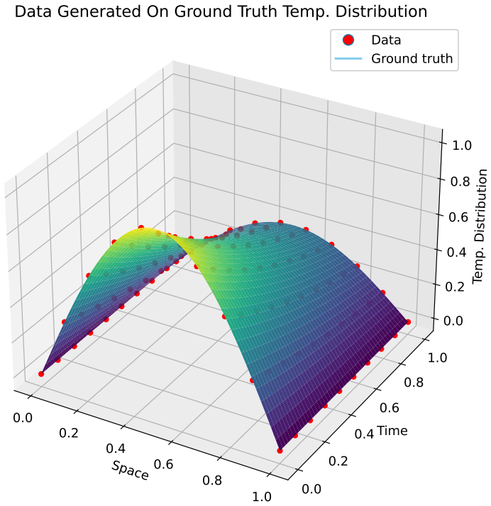
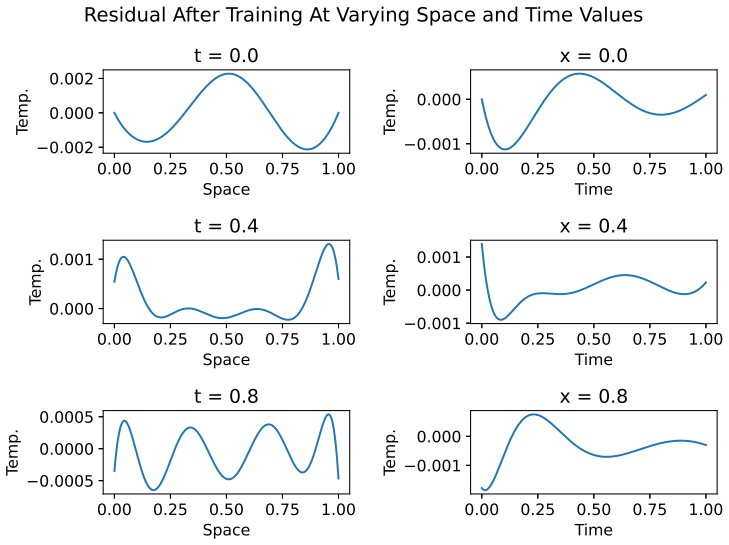
The central claim, stated in the heat-equation results and the conclusion, is that a PINN can solve both the forward and inverse heat equation and is not bound by the CFL condition that governs finite-difference schemes. On the forward problem, the PINN's ground-truth MSE on $[0,1]$ averaged over 10 runs was $2.720\times10^{-6}$; on the inverse problem, adding $D$ as an optimizable parameter gave $D=0.0999$ against the true $0.1$, with MSE $3.774\times10^{-6}$. In the head-to-head test with $\Delta x=\Delta t=0.05$, final time $T=10$, and $D=0.045$ — a combination that violates the CFL condition $D\Delta t\le 0.5(\Delta x)^2$ — the finite-difference solver's MSE jumped to $3.520\times10^{128}$, while the PINN's data-point MSE stayed at $1.558\times10^{-7}$. The authors conclude that the PINN does not have the same accuracy-and-stability requirements as an FDM, because its solution is computed differently from a step-by-step time-marching update.
Load-bearing premise
The load-bearing premise is that the inverse-problem training, starting from a value of $D$ that the paper does not report, finds a minimum that identifies the true thermal diffusivity, with only 100 synthetic points from one wave pattern enough to pin it down.
Editorial extensions
If this is right
- A PINN can fit a PDE solution and identify one of its physical parameters from the same sparse dataset, without a separate inversion step.
- At parameter values that destabilize a finite-difference scheme, the PINN remains usable: with $\Delta x=\Delta t=0.05$, $T=10$, and $D=0.045$, the FDM error was $3.520\times10^{128}$ while the PINN error was $1.558\times10^{-7}$.
- The recovered diffusivity $0.0999$ from data generated with $D=0.1$ indicates that, in this single-mode setup, the decay of one Fourier mode is enough to pin down the parameter.
- Residual weighting matters: $\lambda=0$ overfits, $\lambda=10^{-6}$ follows the data too little outside the training range, and $\lambda=1.0$ gives the best balance between data and physics.
- Denser training data improves the PINN, with average MSE dropping to $2.52\times10^{-9}$ at $\Delta x=\Delta t=0.025$.
Reading between the lines
- The paper does not isolate the mechanism, but the CFL independence likely reflects that the PINN fits a global space-time surface by gradient descent rather than propagating a solution step by step, so the local stability analysis behind CFL does not directly apply; a stress test at longer final times and larger $D$ would map where this independence ends.
- The inverse-problem success may owe much to the data being noise-free, single-mode, and generated from a known analytic form; testing on multi-mode or noisy initial conditions would separate genuine parameter identification from problem simplicity.
- A practical extension is to search numerically for a 'CFL analogue' for the PINN by plotting MSE against $D\Delta t/(\Delta x)^2$ over many configurations; if no threshold appears, that itself suggests grid resolution is not the mechanism limiting PINN accuracy.
Editorial analysis
A structured set of objections, weighed in public.
Referee Report
Summary. This manuscript reports an exploratory study of physics-informed neural networks (PINNs) for solving simple differential equations. The authors construct PINNs for a linear model, a quadratic model, and the one-dimensional heat equation, tune the residual weight λ and the network architecture, and use the heat-equation PINN to recover the thermal diffusivity D from synthetic data. The paper's central claim, stated in Sections 3.3.8 and 5, is that the heat-equation PINN does not share the finite-difference method's (FDM's) Courant–Friedrichs–Lewy (CFL) stability requirement and remains accurate when the FDM becomes unstable.
Significance. If the central claim were quantitatively supported, it would be a useful practical observation about PINN robustness to discretization choices. The inverse-problem demonstration, recovering D = 0.0999 from data generated with D = 0.1, is a reasonable sanity check of a standard PINN capability. The paper also makes an explicit attempt to compare against an FDM baseline across a grid of Δx, Δt, D, and final-time values, which is valuable in principle. However, the significance is substantially undercut by internal inconsistencies: the paper's own appendix contains a CFL-violating case with an order-one PINN error that directly contradicts the conclusion, the PINN and FDM errors are computed on different evaluation sets, and key training details for the inverse problem are omitted. The qualitative toy examples are simple and probably reproducible from the text, but no code is provided and no machine-checked or parameter-free derivation is included.
major comments (4)
- [Section 3.3.8 / Table 23] The conclusion that the PINN 'displayed slight inaccuracies while generally adhering to the input data' when the CFL condition is broken is contradicted by the paper's own Table 23. For Δx = Δt = 0.1, D = 0.09, and T = 100, the reported PINN Data Point MSE is 7.185 × 10^-1. Since the exact solution is bounded by 1 on the domain, this is an order-one error, not a slight inaccuracy. The main text highlights only the T = 10 case (Table 6, MSE 1.558 × 10^-7) and does not mention the T = 100 rows in the appendix, so the support for the load-bearing CFL-robustness claim is incomplete and internally inconsistent.
- [Section 3.3.8 / Tables 6 and 21–29] The comparison between the PINN and the FDM is not apples-to-apples. The column labeled 'PINN Data Point MSE' is evaluated at the sampled training/data points, whereas the FDM MSE is evidently computed over the fully time-marched grid. A small in-sample error does not establish accuracy on the full space-time grid where the FDM comparison is made. To support the claim that the PINN remains accurate under CFL-violating discretizations, the authors need to report PINN error on the same full grid used for the FDM, including off-training points.
- [Table 2] Table 2 reports an overall ground-truth MSE of 2.215 × 10^-1 for the quadratic PINN, with an inside-training-range MSE of 1.495 × 10^-1 over [0,1] and an outside-range MSE of 2.702 × 10^-3 over [-1,0] ∪ [1,2]. Because the outside interval has total length 2 and the inside interval has length 1, the weighted average is approximately (1.495 × 10^-1 + 2 × 2.702 × 10^-3)/3 ≈ 5.16 × 10^-2, not 2.215 × 10^-1. This is arithmetically impossible and indicates that the reported quantitative results need verification.
- [Sections 3.3.3 and 3.3.7] The manuscript contains a literal placeholder in the reported heat-equation training loss: '{Insert Loss after iterations}' appears in Section 3.3.3. More importantly, the inverse-problem claim in Section 3.3.7 is under-specified: the paper does not report the initial value of D, the learning rate, the activation function, or how the boundary and initial conditions are enforced, with Section 3.3.4 merely stating 'we enforced the boundary condition.' Without these details, the recovery of D = 0.0999 from 100 synthetic points could reflect favorable initialization or soft constraint weighting rather than robust identifiability.
minor comments (5)
- [Section 3.2.2] The sentence 'the final optimal network architecture for the Linear PINN was 5 layers and 30 neurons' should refer to the Quadratic PINN, not the Linear PINN.
- [Figure 13] The caption says the model was trained with a '3rd derivative residual loss,' but the text and the equation referenced (Equation 15) describe a fourth-derivative residual.
- [Table 22] The header contains a typo: 'dx=dx=0.1' should be 'dx=dt=0.1'.
- [Section 3.3.6 / Table 4] The explanation of the density parameter is confusing: the text says 'the lower the density the more number of points in our dataset,' which appears to invert the standard meaning of grid density. Please clarify how the datasets for density values 0.1, 0.05, and 0.025 are generated.
- [References] Two references are non-archival web sources (a YouTube video, reference [6], and a blog post, reference [8]); citing the underlying peer-reviewed literature would make the background section more reliable.
Circularity Check
CFL-robustness claim rests on in-sample 'Data Point MSE' (the training objective) and on an architecture selected using the same MSE later reported as performance; the core PINN derivation is otherwise non-circular.
-
fitted input called prediction
[Section 3.3.8, Table 6; Eq. (7); Appendix 7.4 Table 23]
"Ldata = 1 n n∑ i=1 (Yi − ˆYi)2 (7) ... Ltotal = Ldata + λ(Lresidual) (9) ... Table 6 compares the PINN and FDM performance. ... D PINN Data Point MSE FDM MSE ... 0.045 1.558 ∗ 10−7 3.520 ∗ 10128"
Table 6's 'PINN Data Point MSE' is exactly the L_data term of Eq. (7), evaluated on the same synthetic data points used to train the network, and minimizing L_total includes minimizing this term. The paper uses this quantity as the evidence that the PINN 'does not follow the same behavior as the FDM concerning stability and accuracy' past the CFL condition, while the FDM MSE is computed over the fully time-marched grid. The claimed CFL robustness therefore reduces to the fact that the network fits its own training points; it is not an independent accuracy check. The appendix's own Table 23 shows the same metric is 7.185 × 10^-1 at T=100, further contradicting the 'slight inaccuracies' conclusion.
-
fitted input called prediction
[Section 3.3.2 and Table 3]
"we trained the models, calculated the average ground truth MSE on [0, 1] over 5 iterations, and chose the model with the smallest MSE value. ... Average [0,1] Ground Truth MSE 2.720 ∗ 10−6"
The same [0,1] ground-truth MSE is used twice: first as the architecture-selection criterion (the layer/neuron configuration with the smallest MSE is chosen), then as the reported performance metric in Table 3, from which the paper concludes the model 'performed effectively.' The headline accuracy is therefore the minimum over the searched architectures of the evaluation metric, not an unbiased estimate; the favorable result is partly manufactured by the selection procedure.
full rationale
The forward/inverse heat-equation demonstrations are otherwise externally benchmarked: synthetic data are generated from u = e^(-π^2 D t) sin(π x) with D = 0.1, and the reported ground-truth MSEs are compared against that exact solution, so the core PINN derivation is not self-referential. The recovered D = 0.0999 is a genuine inverse-problem output, although the paper omits D's initialization and optimizer settings, which is an identifiability/robustness caveat rather than circularity. No load-bearing self-citation chain appears: reference [12] is used only to motivate future GBM applications. The circularity is concentrated in the evaluation of the central CFL claim: the 'PINN Data Point MSE' is the training objective evaluated on the training points, and the architecture is chosen using the same ground-truth MSE later reported as success. Additionally, the paper's own Appendix Table 23 reports a PINN Data Point MSE of 7.185 x 10^-1 at T=100, an order-one error for a solution bounded by 1, directly contradicting the Conclusion's 'slight inaccuracies while generally adhering to the input data'; this is a correctness inconsistency and metric mismatch independent of the circularity score.
Assumptions & free parameters
free parameters (3)
- residual strength lambda =
1.0 (selected after comparing 1e-6, 1.0, 10.0)
- network architecture (layers, neurons) =
3x20 (linear), 5x30 (quadratic), 5x80 (heat)
- thermal diffusivity D in inverse problem =
0.0999 after training (true value 0.1)
assumptions (5)
- standard math For a degree-n polynomial, the (n+1)-th derivative is identically zero.
- standard math The 1D heat equation with homogeneous Dirichlet boundary conditions has exact solution u(x,t)=e^{-pi^2 D t} sin(pi x).
- domain assumption Minimizing L_data + lambda L_residual over network weights yields an approximate solution of the differential equation and an estimate of its parameters.
- standard math The finite-difference heat-equation scheme is stable only when the CFL condition D*dt <= 0.5*(dx)^2 holds.
- standard math A neural network with enough layers and neurons can approximate the target solution.
Cite this review
Pith. "Pith review of Applications and Manipulations of Physics-Informed Neural Networks in Solving Differential Equations." pith.science (2026). https://pith.science/paper/V6E4HVOP
@misc{pith2026250719522,
  author       = {Pith},
  title        = {Pith review of: Applications and Manipulations of Physics-Informed Neural Networks in Solving Differential Equations},
  year         = {2026},
  howpublished = {\url{https://pith.science/paper/V6E4HVOP}},
  note         = {Machine review of arXiv:2507.19522}
}
read the original abstract
Mathematical models in neural networks are powerful tools for solving complex differential equations and optimizing their parameters; that is, solving the forward and inverse problems, respectively. A forward problem predicts the output of a network for a given input by optimizing weights and biases. An inverse problem finds equation parameters or coefficients that effectively model the data. A Physics-Informed Neural Network (PINN) can solve both problems. PINNs inject prior analytical information about the data into the cost function to improve model performance outside the training set boundaries. This also allows PINNs to efficiently solve problems with sparse data without overfitting by extrapolating the model to fit larger trends in the data. The prior information we implement is in the form of differential equations. Residuals are the differences between the left-hand and right-hand sides of corresponding differential equations; PINNs minimize these residuals to effectively solve the differential equation and take advantage of prior knowledge. In this way, the solution and parameters are embedded into the loss function and optimized, allowing both the weights of the neural network and the model parameters to be found simultaneously, solving both the forward and inverse problems in the process. In this paper, we will create PINNs with residuals of varying complexity, beginning with linear and quadratic models and then expanding to fit models for the heat equation and other complex differential equations. We will mainly use Python as the computing language, using the PyTorch library to aid us in our research.
Figures


Figures from the paper (25 more)






Reference graph
Works this paper leans on
-
[1]
Lecture 6: Finite difference methods
Habib Ammari. “Lecture 6: Finite difference methods”. en. In: ()
-
[2]
Scientific Machine Learning through Physics-Informed Neural Networks: Where we are and What’s next
Salvatore Cuomo et al. Scientific Machine Learning through Physics-Informed Neural Networks: Where we are and What’s next . arXiv:2201.05624 [physics]. June 2022. doi: 10.48550/arXiv.2201.05624 . url: http://arxiv.org/ abs/2201.05624 (visited on 06/26/2024)
-
[3]
Heat Equation: Homogeneous Dirichlet boundary conditions . url: http:// home . iitj . ac . in /~k . r . hiremath / teaching / Lecture - notes - PDEs / node26.html (visited on 06/27/2024)
work page 2024
-
[4]
Machine learning and deep learning
Christian Janiesch, Patrick Zschech, and Kai Heinrich. “Machine learning and deep learning”. en. In: Electronic Markets 31.3 (Sept. 2021), pp. 685–
work page 2021
-
[5]
Diederik P. Kingma and Jimmy Ba. Adam: A Method for Stochastic Opti- mization. arXiv:1412.6980 [cs]. Jan. 2017. doi: 10.48550/arXiv.1412.6980. url: http://arxiv.org/abs/1412.6980 (visited on 07/01/2024)
-
[6]
url: https://www.youtube.com/watch?v=G_hIppUWcsc
Physics-Informed Neural Networks (PINNs) - An Introductio n - Ben Moseley — Jousef Murad . url: https://www.youtube.com/watch?v=G_hIppUWcsc. 47
-
[7]
Deep learning in neural networks: An ov erview
J¨ urgen Schmidhuber. “Deep learning in neural networks: An ov erview”. In: Neural Networks 61 (Jan. 2015), pp. 85–117. issn: 0893-6080. doi: 10 . 1016/j.neunet.2014.09.003 . url: https://www.sciencedirect.com/ science/article/pii/S0893608014002135 (visited on 06/28/2024)
work page 2015
-
[8]
So, what is a physics-informed neural network? - Ben Moseley . url: https: //benmoseley.blog/my- research/so- what- is- a- physics- informed- neural-network/ (visited on 06/26/2024)
work page 2024
Show all 13 references
-
[9]
A comprehensive survey on regular ization strategies in machine learning
Yingjie Tian and Yuqi Zhang. “A comprehensive survey on regular ization strategies in machine learning”. In: Information Fusion 80 (Apr. 2022), pp. 146–166. issn: 1566-2535. doi: 10.1016/j.inffus.2021.11.005 . url: https://www.sciencedirect.com/science/article/pii/S15662535210...
2022 doi
-
[10]
What is Adam Optimizer? en
Neha Vishwakarma. What is Adam Optimizer? en. Sept. 2023. url: https: //www.analyticsvidhya.com/blog/2023/09/what-is-adam -optimizer/ (visited on 07/01/2024)
2023
-
[11]
Physics-informed Neural Networks: a simple tutorial with P y- Torch
Theo Wolf. Physics-informed Neural Networks: a simple tutorial with P y- Torch. en. Jan. 2024. url: https://medium.com/@theo.wolf/physics- informed-neural-networks-a-simple-tutorial-with-pyt orch-f28a890b874a (visited on 06/26/2024)
2024
-
[12]
Personalized Predictions of Glioblastoma Infiltra- tion: Mathematical Models, Physics-Informed Neural Netwo rks and Multi- modal Scans
Ray Zirui Zhang et al. Personalized Predictions of Glioblastoma Infiltra- tion: Mathematical Models, Physics-Informed Neural Netwo rks and Multi- modal Scans. arXiv:2311.16536 [cs, eess, q-bio]. Jan. 2024. doi: 10.48550/ arXiv.2311.16536. url: http://arxiv.org/abs/2311.16536 (v...
-
[695]
doi: 10.1007/s12525- 021- 00475- 2
issn: 1422-8890. doi: 10.1007/s12525- 021- 00475- 2 . url: https: //doi.org/10.1007/s12525-021-00475-2 (visited on 06/28/2024)
2024 doi
Reviewed August 6, 2026 · model on record in the stance chip above.
Discussion (0). Sign in to comment.