REVIEW 3 major objections 5 minor 72 references
Visual Analytics Using Tensor Unified Linear Comparative Analysis
T0 review · 3 major / 5 minor · reviewed 2026-08-06 · deepseek-v4-flash
Pith's one-line read TULCA is a tensor decomposition method that unifies discriminant analysis and contrastive learning, letting analysts compare tensor groups while preserving or suppressing group-specific variance.
desk verdict TULCA is a well-specified tensor extension of ULCA with a real gap-filler in TcPCA and convincing, honest case studies; the untested per-mode factorization assumption is the main caveat but not a dealbreaker. read the letter →
The pith
A machine-rendered reading of the paper's core claim, the machinery that carries it, and where it could break.
The reading
What carries the argument
The load-bearing object is the per-mode trace-ratio optimization in Eq. 11. For each mode n (n >= 2), TULCA constructs two matrices C_a^(n) and C_b^(n) from mode-n matricizations of the tensor, using group labels along mode-1: C_a^(n) aggregates target within-class covariances and between-class covariances with target weights w_tg^(n) and between-class weights w_bw^(n), while C_b^(n) aggregates background within-class covariances with background weights w_bg^(n). The projection matrix M_n is the maximizer of the trace ratio, solved by iterative eigenvalue decomposition; the projections are then applied through n-mode products to form the core tensor. The weight parameters act as a dial that moves the method continuously between discriminant analysis and contrastive learning. To visualize the N-mode core tensor, the method applies CP decomposition and displays the first two mode-1 factors as a 2D scatterplot and the associated factors of other modes as bar charts.
What would settle it
Construct a third-order tensor whose group labels are separated only by a rank-1 pattern that spans multiple modes, such as a time pattern times an instance pattern times a variable pattern, with no marginal difference visible in any single mode's matricization. If TULCA with discriminant-analysis weights fails to separate the groups in the core tensor while a jointly optimized multilinear projection succeeds, the independent per-mode optimization is the bottleneck.
Extended reading notes
Core claim
The paper's central claim is that TULCA is the first tensor decomposition method that supports contrastive learning, and that by integrating discriminant analysis and contrastive learning it enables flexible comparison of tensors. In the method, for each mode n the projection matrix M_n maximizes the trace-ratio tr(M_n^T C_a^(n) M_n)/tr(M_n^T C_b^(n) M_n), where C_a^(n) is a weighted sum of within-class and between-class covariance matrices of group l and C_b^(n) is a weighted sum of background within-class covariances, with weights chosen by the analyst; applying all projections via n-mode products yields the core tensor. Setting the weights appropriately reproduces TDA, a tensor cPCA (TcPCA), or simultaneous separation and variance preservation, as demonstrated on synthetic data and on supercomputer and mobile-health logs.
Load-bearing premise
The load-bearing premise is that optimizing each mode's projection independently, on covariance matrices computed from mode-n matricizations defined by mode-1 group labels, captures the group comparison of interest; if the comparative structure lives in interactions among modes, this per-mode optimization could miss it.
Editorial extensions
If this is right
- Analysts can now compare tensor groups in one decomposition that separates groups and preserves (or suppresses) group-specific variance, a combination no previous tensor decomposition offered.
- TULCA reproduces TDA and a tensor extension of cPCA (TcPCA) as special cases of its weight settings, so a single implementation covers both contrastive and discriminant analyses.
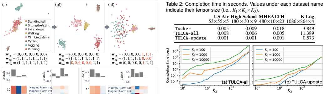
- Because covariance matrices are precomputed once, updating the weights for interactive steering only requires re-solving the per-mode trace-ratio problem; on the K computer log dataset the update took under a second.
- The CP-based core-tensor visualization turns an N-mode core tensor into one 2D scatterplot plus 2(N-1) bar charts, making the results interpretable in a visual analytics workflow.
- In the case studies, the method identified cooling-infrastructure changes and sensor failures in supercomputer logs, and differentiated jogging, running, and cycling in mobile-health sensor data.
Reading between the lines
- A natural extension not tested in the paper is joint optimization of all mode projection matrices, such as alternating or coupled optimization, to capture comparative structure that appears only through cross-mode interactions; the independent per-mode optimization is the likeliest place this would matter.
- The weight parameters could be learned from analyst demonstrations rather than tuned by hand: the paper cites backward parameter selection for ULCA as a route where an analyst shows a desired scatterplot arrangement and the system infers weights.
- For tensors with many groups or modes, the interface's parameter view and per-mode bar charts would need a hierarchical or aggregated design, which the paper itself flags as future work.
- The contrastive-learning capability could be tested on other multivariate spatiotemporal domains, such as network traffic or climate sensor arrays, where group-specific salient patterns are the analysis target.
Signed reviews
Editorial analysis
A structured set of objections, weighed in public.
Referee Report
Summary. The paper introduces TULCA (tensor unified linear comparative analysis), a tensor decomposition method that extends ULCA from matrices to high-order tensors. The method solves a trace-ratio optimization per mode, using weighted within-class, between-class, and background covariance matrices computed from mode-n matricizations, then projects all non-comparison modes via n-mode products to form a core tensor. The authors also propose a CP-based visualization scheme for the core tensor and integrate it into an interactive visual analytics interface. The method is evaluated with synthetic data, two real-world case studies (K computer operational logs and MHEALTH physical-activity data), and runtime benchmarks against Tucker decomposition, with an additional qualitative comparison against ULCA applied to matricized tensors.
Significance. If the claims hold, TULCA fills a real gap: existing tensor decomposition methods do not support contrastive learning, and the ability to blend discriminant and contrastive objectives in one tensor decomposition is useful for visual analytics. The strengths of the paper include a clearly specified optimization, an efficient update strategy that pre-computes covariance matrices, public source code, a sensible core-tensor visualization design, and domain-expert feedback from a realistic supercomputer-log analysis scenario. However, the central claim of "flexible comparison of tensors" relies on an untested factorization assumption, and the quantitative evaluation is limited to runtime, with no objective quality metric comparing TULCA against existing tensor discriminant or contrastive methods. These issues are load-bearing for the novelty and scope claims, so the paper needs further work before it can be accepted.
major comments (3)
- [Sec. 3.2.2, Eqs. (11)-(13)] The construction solves Eq. (11) independently for each mode using only the mode-n covariance matrices C^(n)_wil and C^(n)_bwl. This assumes that all group-relevant structure is visible in the marginal mode-n covariances. A counterexample shows the limitation: for two groups of 2x2 slices with orthonormal factor matrices A and B, Group 1 having coefficient matrix diag(u_t,v_t) and Group 2 having [[0,u_t],[v_t,0]] with i.i.d. u_t,v_t and E[u_t^2]=E[v_t^2], the mode-2 and mode-3 covariance matrices are identical across groups even though the multilinear association structure differs. In this regime Eq. (11) gives no contrastive preference, so TULCA cannot separate the groups. The synthetic experiment in Sec. 5 and the case studies in Sec. 6 use patterns that are visible in marginal covariances, so they do not exercise this failure mode. The authors should either add an experiment with a cross-mode interaction pattern of this kind and report the resulting behavior, or explicitly state and discuss this factorization assumption as a limitation of the claim that TULCA enables flexible comparison of tensors.
- [Sec. 5 and Sec. 8] The evaluation is almost entirely qualitative. The synthetic experiment in Sec. 5 is assessed visually, and the comparison in Sec. 8 against ULCA is qualitative despite the text in the first sentence of Sec. 8 saying "We quantitatively compare." The only quantitative results are runtimes in Table 2 and Fig. 10. The paper claims to demonstrate TULCA's efficacy, but there is no objective measure of separation quality, variance preservation, or contrastive fidelity, and no quantitative comparison with tensor discriminant analysis (TDA) or a tensor extension of cPCA obtained by matricization. Please add objective metrics for the synthetic and case-study settings (e.g., silhouette scores, classification accuracy, or a between/within variance ratio) and compare TULCA against at least TDA and a matricized-cPCA baseline, or soften the efficacy claims accordingly.
- [Sec. 4.2 and Sec. 9] The visualization pipeline and the parameter sensitivity are not fully validated. The core-tensor visualization in Sec. 4.2 relies on CP decomposition with a default rank R=2, but CP decomposition is subject to scaling and permutation indeterminacy, and the paper does not discuss how sign ambiguity or component ordering affects the scatterplot and bar-chart interpretation. The authors themselves note in Sec. 9 that weight parameter selection requires trial-and-error and can produce spurious visual patterns, but no sensitivity analysis is provided. For a method whose central contribution is interactive steering, a brief sensitivity study showing how stable the core tensor is under small weight changes would substantially strengthen the claims.
minor comments (5)
- [Sec. 3.1.2] Equation (1) says "identify matrix"; this should be "identity matrix."
- [Sec. 6.1] The phrase "third-core tensor" should be "third-order tensor."
- [Sec. 7 and Table 2] There are typographical inconsistencies: "TULCA-all" is spelled "TUCLA-all" in the text and table header at several points; please unify the spelling.
- [Sec. 8] The first sentence says "We quantitatively compare TULCA and ULCA results," but the section title is "Qualitative Comparison" and the described evaluation is qualitative. Please correct the wording.
- [Fig. 6] The caption contains a typo: "respecively" should be "respectively."
Circularity Check
TULCA extends ULCA per-mode without fitting; the reported comparisons are demonstrations and case studies, not predictions forced by construction.
full rationale
The derivation chain is self-contained and not circular. TULCA's optimization (Eqs. 11-13) is a direct mode-wise generalization of ULCA (Eqs. 8-10), with covariance matrices defined from mode-n matricizations (Eqs. 6-7) and the core tensor obtained by n-mode products (Eq. 4). The weight parameters are interactive analyst inputs, not fitted to data; no quantity is estimated from a subset and then reported as a prediction. The synthetic experiments and case studies are exploratory demonstrations validated by known data structure or domain-expert feedback, not statistical predictions that reduce to the method's inputs by construction. The heavy citation to the authors' prior ULCA is used for the optimization solver and DR formulation, but the tensor extension itself is defined in this paper and is not identical to matrix ULCA; the centrality of the tensor contribution therefore does not rest on an unverified self-citation chain. Accordingly, no circular step is identified.
Assumptions & free parameters
free parameters (3)
- Weight parameters wtgl, wbgl, wbwl per group and mode =
user-set in [0,1], default equal across modes
- Number of components K'_n per mode =
user-set (e.g., 2x3 in synthetic experiments)
- CP rank R for core visualization =
R=2 by default
assumptions (3)
- domain assumption Groups are defined along the first mode, and other modes are compressed (Sec. 3.1.2).
- domain assumption Optimizing each mode's projection independently via Eq. 11 and applying n-mode products yields a useful comparative core tensor.
- standard math The trace-ratio problem (Eq. 11) can be solved by iterative eigenvalue decomposition, given automatic regularization when denominators vanish.
Cite this review
Pith. "Pith review of Visual Analytics Using Tensor Unified Linear Comparative Analysis." pith.science (2026). https://pith.science/paper/BPCY4YLT
@misc{pith2026250719988,
  author       = {Pith},
  title        = {Pith review of: Visual Analytics Using Tensor Unified Linear Comparative Analysis},
  year         = {2026},
  howpublished = {\url{https://pith.science/paper/BPCY4YLT}},
  note         = {Machine review of arXiv:2507.19988}
}
read the original abstract
Comparing tensors and identifying their (dis)similar structures is fundamental in understanding the underlying phenomena for complex data. Tensor decomposition methods help analysts extract tensors' essential characteristics and aid in visual analytics for tensors. In contrast to dimensionality reduction (DR) methods designed only for analyzing a matrix (i.e., second-order tensor), existing tensor decomposition methods do not support flexible comparative analysis. To address this analysis limitation, we introduce a new tensor decomposition method, named tensor unified linear comparative analysis (TULCA), by extending its DR counterpart, ULCA, for tensor analysis. TULCA integrates discriminant analysis and contrastive learning schemes for tensor decomposition, enabling flexible comparison of tensors. We also introduce an effective method to visualize a core tensor extracted from TULCA into a set of 2D visualizations. We integrate TULCA's functionalities into a visual analytics interface to support analysts in interpreting and refining the TULCA results. We demonstrate the efficacy of TULCA and the visual analytics interface with computational evaluations and two case studies, including an analysis of log data collected from a supercomputer.
Figures


Figures from the paper (7 more)




Reference graph
Works this paper leans on
-
[1]
https://github.com/vizlab-kobe/tulca
The supplementary materials: The source code for TULCA and the evaluations, along with a demonstration video of the visual interface. https://github.com/vizlab-kobe/tulca. 2, 6
-
[2]
A. Abid, M. J. Zhang, V . K. Bagaria, and J. Zou. Exploring patterns enriched in a dataset with contrastive principal component analysis. Nat Commun, 9(1):2134, 2018. doi: 10.1038/s41467-018-04608-8 1, 2
-
[3]
S. Adibi. Mobile Health: A Technology Road Map, vol. 5. Springer, 2015. doi: 10.1007/978-3-319-12817-7 6
-
[4]
N. Andrienko and G. Andrienko. A visual analytics framework for spatio- temporal analysis and modelling. Data Min Knowl Discov , 27:55–83,
-
[5]
N. Andrienko, G. Andrienko, and P. Gatalsky. Exploratory spatio-temporal visualization: An analytical review. J Visual Lang Comput, 14(6):503–541,
-
[6]
O. Banos, R. Garcia, J. A. Holgado-Terriza, M. Damas, H. Pomares, et al. mHealthDroid: A novel framework for agile development of mobile health applications. In L. Pecchia, L. L. Chen, C. Nugent, and J. Bravo, eds., Ambient Assisted Living and Daily Activities, pp. 91–98. Springer, 2014. doi: 10.1007/978-3-319-13105-4_14 7
- [7]
-
[8]
P. Boileau, N. S. Hejazi, and S. Dudoit. Exploring high-dimensional bio- logical data with sparse contrastive principal component analysis. Bioin- formatics, 36(11):3422–3430, 2020. doi: 10.1093/bioinformatics/btaa176 2
Show all 72 references
-
[9]
Brandt, F
J. Brandt, F. Ciorba, A. Gentile, M. Ott, and T. Wilde. Driving HPC oper- ations with holistic monitoring and operational data analytics (Dagstuhl Seminar 23171). Dagstuhl Reports, 13(4):98–120, 2023. doi: 10.4230/ DagRep.13.4.98 1
2023
-
[10]
N. Cao, C. Lin, Q. Zhu, Y .-R. Lin, X. Teng, and X. Wen. V oila: Visual anomaly detection and monitoring with streaming spatiotemporal data. IEEE Trans Vis Comput Graph, 24(1):23–33, 2018. doi: 10.1109/TVCG. 2017.2744419 3
2018
-
[11]
Eckart–Young
J. D. Carroll and J.-J. Chang. Analysis of individual differences in multidi- mensional scaling via an N-way generalization of “Eckart–Young” decom- position. Psychometrika, 35(3):283–319, 1970. doi: 10.1007/BF02310791 2
1970 doi
-
[12]
Chari and L
T. Chari and L. Pachter. The specious art of single-cell genomics. PLOS Comput Biol, 19(8):e1011288, 2023. 20 pages. doi: 10.1371/journal.pcbi. 1011288 9
2023 doi
-
[13]
Clemmensen, T
L. Clemmensen, T. Hastie, D. Witten, and B. Ersbøll. Sparse discriminant analysis. Technometrics, 53(4):406–413, 2011. doi: 10.1198/TECH.2011. 08118 2
2011 doi
-
[14]
J. P. Cunningham and Z. Ghahramani. Linear dimensionality reduction: Survey, insights, and generalizations.J Mach Learn Res, 16(1):2859–2900,
-
[15]
Fournet and A
J. Fournet and A. Barrat. Contact patterns among high school students. PLOS One, 9(9), 2014. doi: 10.1371/journal.pone.0107878 8
2014 doi
-
[16]
Fujita, N
K. Fujita, N. Sakamoto, T. Fujiwara, T. Tsukamoto, and J. Nonaka. A visual analytics method for time-series log data using multiple dimen- sionality reduction. J Adv Simul Sci Eng , 9(2):206–219, 2022. doi: 10. 15748/jasse.9.206 3
2022
-
[17]
Fujiwara, O.-H
T. Fujiwara, O.-H. Kwon, and K.-L. Ma. Supporting analysis of dimension- ality reduction results with contrastive learning. IEEE Trans Vis Comput Graph, 26(1):45–55, 2020. doi: 10.1109/TVCG.2019.2934251 1, 2
2020
-
[18]
https://jmlr.org/papers/volume16/cunningham15a/cunningham15a. pdf. 2
-
[19]
Fujiwara, Shilpika, N
T. Fujiwara, Shilpika, N. Sakamoto, J. Nonaka, K. Yamamoto, and K.- L. Ma. A visual analytics framework for reviewing multivariate time- series data with dimensionality reduction. IEEE Trans Vis Comput Graph, 27(2):1601–1611, 2021. doi: 10.1109/TVCG.2020.3028889 2, 3, 8
2021
-
[20]
Fujiwara, X
T. Fujiwara, X. Wei, J. Zhao, and K.-L. Ma. Interactive dimensional- ity reduction for comparative analysis. IEEE Trans Vis Comput Graph, 28(1):758–768, 2022. doi: 10.1109/TVCG.2021.3114807 1, 2, 4, 5, 9
2022
-
[21]
Ge and J
R. Ge and J. Zou. Rich component analysis. In Proc. ICML, pp. 1502– 1510, 2016. https://proceedings.mlr.press/v48/gea16.html. 2
2016
-
[22]
Fujiwara and T.-P
T. Fujiwara and T.-P. Liu. Contrastive multiple correspondence analysis (cMCA): Using contrastive learning to identify latent subgroups in political parties. PLOS ONE, 18(7):e0287180, 2023. doi: 10.1371/journal.pone. 0287180 2
2023 doi
-
[23]
Golkar, D
S. Golkar, D. Lipshutz, T. Tesileanu, and D. B. Chklovskii. An online algorithm for contrastive principal component analysis. In Proc. ICASSP, pp. 1–5. IEEE, 2023. doi: 10.1109/ICASSP49357.2023.10096380 2
2023
-
[24]
Y . Guo, T. Hastie, and R. Tibshirani. Regularized linear discriminant analysis and its application in microarrays. Biostatistics, 8(1):86–100,
-
[25]
C. Hare, D. A. Armstrong, R. Bakker, R. Carroll, and K. T. Poole. Using bayesian Aldrich-McKelvey scaling to study citizens’ ideological pref- erences and perceptions. Am J Polit Sci, 59(3):759–774, 2015. doi: 10. 2139/ssrn.3375435 1
2015
-
[26]
Gleicher
M. Gleicher. Explainers: Expert explorations with crafted projections. IEEE Trans Vis Comput Graph, 19(12):2042–2051, 2013. doi: 10.1109/ TVCG.2013.157 1
2013
-
[27]
A. J. Izenman. Linear discriminant analysis. In Modern Multivariate Statistical Techniques: Regression, Classification, and Manifold Learning, pp. 237–280. Springer, 2013. doi: 10.1007/978-0-387-78189-1 2, 3
2013 doi
-
[28]
H. Jeon, H. Lee, Y .-H. Kuo, T. Yang, D. Archambault, et al. Unveiling high-dimensional backstage: A survey for reliable visual analytics with dimensionality reduction. In Proc CHI. ACM, New York, 2025. doi: 10. 1145/3706598.3713551 9
2025
-
[29]
I. T. Jolliffe. Principal Component Analysis. Springer Series in Statistics. Springer, 2002. doi: 10.1007/b98835 2
2002 doi
-
[30]
Kaya and B
O. Kaya and B. Uçar. High performance parallel algorithms for the Tucker decomposition of sparse tensors. In Proc. ICPP, pp. 103–112. IEEE, 2016. 9
2016
-
[31]
explanatory
R. A. Harshman. Foundations of the PARAFAC procedure: Models and conditions for an “explanatory” multi-mode factor analysis. UCLA Working Papers in Phonetics, 16:1–84, 1970. 2
1970
-
[32]
H. A. Kiers. Towards a standardized notation and terminology in multiway analysis. J Chemom, 14(3):105–122, 2000. doi: 10.1002/1099-128X (200005/06)14:3<105::AID-CEM582>3.0.CO;2-I 2
2000 doi
-
[33]
T. G. Kolda and B. W. Bader. Tensor decompositions and applications. SIAM Rev, 51(3):455–500, 2009. doi: 10.1137/07070111X 1, 3, 6
2009 doi
-
[34]
Kossaifi, Y
J. Kossaifi, Y . Panagakis, A. Anandkumar, and M. Pantic. TensorLy: Tensor learning in python. J Mach Learn Res, 20(26):1–6, 2019. http: //jmlr.org/papers/v20/18-277.html. 4
2019
-
[35]
Z. Lai, Y . Xu, J. Yang, J. Tang, and D. Zhang. Sparse tensor discriminant analysis. IEEE Trans Image Process, 22(10):3904–3915, 2013. doi: 10. 1109/TIP.2013.2264678 2, 3
2013
-
[36]
H. A. Kiers. Hierarchical relations among three-way methods. Psychome- trika, 56(3):449–470, 1991. doi: 10.1007/BF02294485 2
1991 doi
-
[37]
D. Liu, P. Xu, and L. Ren. TPFlow: Progressive partition and multidi- mensional pattern extraction for large-scale spatio-temporal data analysis. IEEE Trans Vis Comput Graph, 25(1):1–11, 2019. doi: 10.1109/TVCG. 2018.2865018 1, 2, 3
2019
-
[38]
H. Lu, K. N. Plataniotis, and A. N. Venetsanopoulos. A survey of multilin- ear subspace learning for tensor data. Pattern Recognit, 44(7):1540–1551,
-
[39]
Lu, S.-H
R.-S. Lu, S.-H. Wang, and S.-Y . Huang. A geometric algorithm for contrastive principal component analysis in high dimension. J Comput Graph Stat, pp. 1–8, 2024. doi: 10.1080/10618600.2023.2289542 2
2024
- [40]
-
[41]
P. H. Le-Khac, G. Healy, and A. F. Smeaton. Contrastive representation learning: A framework and review. IEEE Access, 8:193907–193934, 2020. doi: 10.1109/ACCESS.2020.3031549 2
2020
-
[42]
I. V . Oseledets. Tensor-train decomposition. SIAM J Sci Comput , 33(5):2295–2317, 2011. doi: 10.1137/090752286 1
2011 doi
-
[43]
M. Ott, W. Shin, N. Bourassa, T. Wilde, S. Ceballos, et al. Global expe- riences with HPC operational data measurement, collection and analysis. In Proc. CLUSTER, pp. 499–508, 2020. doi: 10.1109/CLUSTER49012. 2020.00071 1
2020
-
[44]
Pajarola, S
R. Pajarola, S. K. Suter, R. Ballester-Ripoll, and H. Yang. Tensor approxi- mation for multidimensional and multivariate data. In Anisotropy Across Fields and Scales, pp. 73–98. Springer, 2021. doi: 10.1007/978-3-030 -56215-1_4 2
2021 doi
-
[45]
Dash Python user guide
Plotly. Dash Python user guide. https://dash.plotly.com/, 2024. Accessed: 2024-09-22. 6
2024
-
[46]
Rabanser, O
S. Rabanser, O. Shchur, and S. Günnemann. Introduction to tensor decom- 10 To appear in IEEE Transactions on Visualization and Computer Graphics. positions and their applications in machine learning. arXiv:1711.10781,
-
[47]
Miyazaki, Y
H. Miyazaki, Y . Kusano, N. Shinjou, F. Shoji, M. Yokokawa, and T. Watan- abe. Overview of the K computer system. Fujitsu Sci Tech J, 48(3):255– 265, 2012. 6
2012
-
[48]
D. Tao, X. Li, X. Wu, and S. J. Maybank. General tensor discriminant analysis and Gabor features for gait recognition. IEEE Trans Pattern Anal Mach Intell, 29(10):1700–1715, 2007. doi: 10.1109/TPAMI.2007.1096 2
2007
-
[49]
J. B. Tenenbaum, V . d. Silva, and J. C. Langford. A global geometric frame- work for nonlinear dimensionality reduction. Science, 290(5500):2319– 2323, 2000. doi: 10.1126/science.290.5500.2319 2
-
[50]
M. E. Timmerman and H. A. Kiers. Three-mode principal compo- nents analysis: Choosing the numbers of components and sensitivity to local optima. Br J Stat Psychol , 53(1):1–16, 2000. doi: 10.1348/ 000711000159132 9
-
[51]
Townsend, N
J. Townsend, N. Koep, and S. Weichwald. Pymanopt: A Python toolbox for optimization on manifolds using automatic differentiation. J Mach Learn Res, 17(137):1–5, 2016. https://jmlr.org/papers/v17/16-177.html. 4
2016
-
[52]
L. R. Tucker. Some mathematical notes on three-mode factor analysis. Psychometrika, 31(3):279–311, 1966. doi: 10.1007/BF02289464 1, 2
1966 doi
-
[53]
Air Data: Air quality data collected at outdoor monitors across the US
US Environmental Protection Agency. Air Data: Air quality data collected at outdoor monitors across the US. https://www.epa.gov/ outdoor-air-quality-data, 2019. Accessed: 2024-09-23. 8
2019
-
[54]
Salloum and C.-C
R. Salloum and C.-C. J. Kuo. cPCA++: An efficient method for contrastive feature learning. Pattern Recognit, 124:108378, 2022. doi: 10.1016/j. patcog.2021.108378 2
2022
-
[55]
van der Maaten, E
L. van der Maaten, E. Postma, and J. van den Herik. Dimensionality reduc- tion: A comparative review. Technical Report TiCC-TR 2009-005, Tilburg University Technical Report, 2009. 36 pages, https://lvdmaaten.github.io/ publications/papers/TR_Dimensionality_Reduction_Review_2009.pdf. 2
2009
-
[56]
Virtanen, R
P. Virtanen, R. Gommers, T. E. Oliphant, M. Haberland, T. Reddy, et al. SciPy 1.0: Fundamental algorithms for scientific computing in Python. Nat Methods, 17:261–272, 2020. doi: 10.1038/s41592-019-0686-2 4
2020 doi
-
[57]
Y . Wang, H. Huang, C. Rudin, and Y . Shaposhnik. Understanding how dimension reduction tools work: An empirical approach to deciphering t- SNE, UMAP, TriMAP, and PaCMAP for data visualization.J Mach Learn Res, 22(201):1–73, 2021. https://www.jmlr.org/papers/v22/20-1061.html. 9
2021
-
[58]
Z. Wang, H. Xiong, J. Zhang, S. Yang, M. Boukhechba, et al. From personalized medicine to population health: A survey of mhealth sensing techniques. IEEE Internet Things J, 9(17):15413–15434, 2022. doi: 10. 1109/JIOT.2022.3161046 1
2022
-
[59]
J. Wen, X. Fang, J. Cui, L. Fei, K. Yan, et al. Robust sparse linear discriminant analysis. IEEE Trans Circ Syst Video Tech, 29(2):390–403,
-
[60]
S. Yan, D. Xu, Q. Yang, L. Zhang, X. Tang, and H.-J. Zhang. Discriminant analysis with tensor representation. In Proc. CVPR, vol. 1, pp. 526–532. IEEE, 2005. doi: 10.1109/CVPR.2005.131 2
2005 doi
-
[61]
van der Maaten and G
L. van der Maaten and G. Hinton. Visualizing data using t-SNE. J Mach Learn Res, 9(11), 2008. https://jmlr.org/papers/v9/vandermaaten08a.html. 2
2008
-
[62]
J. Yang, D. Zhang, X. Yong, and J.-y. Yang. Two-dimensional discriminant transform for face recognition. Pattern Recognit, 38(7):1125–1129, 2005. doi: 10.1016/j.patcog.2004.11.019 2, 8, 9
2005 doi
-
[63]
Yasir, E
M. Yasir, E. Angelakis, F. Bibi, E. Azhar, D. Bachar, et al. Comparison of the gut microbiota of people in France and Saudi Arabia. Nutr Diabetes, 5(4):e153–e153, 2015. doi: 10.1038/nutd.2015.3 1
2015 doi
-
[64]
J. Y . Zou, D. J. Hsu, D. C. Parkes, and R. P. Adams. Con- trastive learning using spectral methods. In Proc. NIPS , pp. 2238–2246, 2013. https://papers.nips.cc/paper_files/paper/2013/hash/ 36a16a2505369e0c922b6ea7a23a56d2-Abstract.html. 2 11
2013
-
[69]
J. Yang, D. Zhang, A. F. Frangi, and J.-y. Yang. Two-dimensional PCA: A new approach to appearance-based face representation and recognition. IEEE Trans Pattern Anal Mach Intell , 26(1):131–137, 2004. doi: 10. 1109/TPAMI.2004.1261097 2, 8, 9
2004 arXiv
-
[2003]
doi: 10.1016/S1045-926X(03)00046-6 2
-
[2007]
doi: 10.1093/biostatistics/kxj035 2, 4
-
[2011]
doi: 10.1016/j.patcog.2011.01.004 1
2011 doi
-
[2013]
doi: 10.1007/s10618-012-0285-7 2
-
[2015]
doi: 10.1186/1475-925X-14-S2-S6 1, 7
-
[2017]
doi: 10.48550/arXiv.1711.1078 2
-
[2018]
doi: 10.1109/TCSVT.2018.2799214 2
2018
Reviewed August 6, 2026 · model on record in the stance chip above.
Discussion (0). Continue with ORCID to comment.