REVIEW 3 major objections 5 minor 76 references
Fourier space readout method for efficiently recovering functions encoded in quantum states
T0 review · 3 major / 5 minor · reviewed 2026-08-15 · deepseek-v4-flash
Pith's one-line read Reading out a quantum-encoded function can be done with shots set by smoothness, not grid size.
desk verdict The core idea is clean and the numerics are persuasive, but the paper's headline claim of N-independent readout cost is not actually proven because the sign-determination step sits outside the formal error analysis. read the letter →
The pith
A machine-rendered reading of the paper's core claim, the machinery that carries it, and where it could break.
The reading
What carries the argument
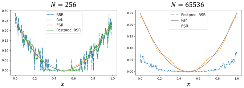
The central object is the even-extension operator followed by the inverse quantum Fourier transform. The extension operator doubles the computational domain and makes the amplitude-encoded function center-symmetric, so the resulting quantum Fourier coefficients are real-valued; post-selecting the high-order register leaves only the $M$ dominant coefficients. Their magnitudes come from one Z-basis circuit, and their signs come from a second circuit built with a linear combination of unitaries that shifts the state by a known constant. This carries the argument because the Fourier coefficients of a smooth function decay as $O(k^{-p})$, so $M=O((1/\varepsilon)^{2/(2p-1)})$ suffices and the total shot count becomes $O((1/\varepsilon)^{2+2/(2p-1)})$, independent of $N$.
What would settle it
Take a discontinuous or endpoint-mismatched function and run the FSR circuits at a fixed shot count; for instance, compare the RMSE for $f(x)=x^2$ with $f(x)=\operatorname{sign}(\sin(2\pi x))$ at $N=1024$ and $N=65536$. If the RMSE grows with $N$, or if the inferred $M$ must grow with $N$ rather than with $(1/\varepsilon)^s$, the central $N$-independence claim is wrong.
Extended reading notes
Core claim
The paper claims that for a real-valued function $f$ amplitude-encoded as $\psi_j = f(jL/N)/A_N$, the inverse quantum Fourier transform followed by post-selection yields all $M$ dominant Fourier coefficients at once: their absolute values from one measurement circuit and their signs from an LCU-shift circuit. Because the Fourier coefficients of a regular function decay, $M=O((1/\varepsilon)^s)$ terms suffice for error $\varepsilon$, and the measurement repetition count is $O((1/\varepsilon)^{2+s})$ — both independent of the grid number $N$. The classical reconstruction $f(x)\approx (A_N/\sqrt{N})(\hat c_0+2\sum_{k=1}^{M-1}\hat c_k \cos(k\pi x/L))$ costs $O(JM)$ for $J$ target points. The paper concludes that readout of function-based quantum states does not ruin the quantum speedup regarding grid number.
Load-bearing premise
The central grid-number independence rests on the input function having Fourier coefficients that decay quickly enough that a fixed number $M$, set only by the desired error, captures it; for rough, oscillatory, or discontinuous functions the necessary $M$ grows with the grid and the shot count loses its $N$-independence.
Editorial extensions
If this is right
- For smooth, boundary-matched solutions of PDEs, the shot count needed to read out the full solution becomes independent of the grid number, so the quantum solver's speedup in $N$ is no longer cancelled by readout.
- When only $J$ target points matter, classical reconstruction costs $O(J(1/\varepsilon)^s)$ plus the histogram cost, so targeted regions of the solution can be extracted much more cheaply than all $N$ grid values.
- The $N_{\mathrm{shot}}$-adaptive scheme lets the algorithm choose the truncation $M$ from the measurement record alone, removing the need to know the function in advance.
- The $d$-dimensional version uses $d+1$ ancillary qubits and tensorized circuits, giving the same independence of $N$ in each dimension.
- Even and odd extension operators handle periodic and zero-boundary cases, and reconstruction is defined at arbitrary target points, not only at the grid points.
Reading between the lines
- Beyond the paper, the argument is a compression argument: any basis with a cheap unitary quantum transform and sparse or decaying coefficients for the solution class, such as wavelets, should inherit the same readout scaling; the paper itself notes Chebyshev transforms but flags the difficulty of constructing a unitary inverse.
- Beyond the paper, the adaptive truncation rule could serve as a built-in spectral-error indicator: if non-negligible coefficients still appear near the cutoff as the shot count grows, the simulation is under-resolved at that scale.
- A testable extension is to push the method to solutions with shocks or interfaces; one would expect a crossover in $N$ beyond which the FSR error starts growing, and a piecewise or dictionary basis might restore $N$-independence.
Signed reviews
Editorial analysis
A structured set of objections, weighed in public.
Referee Report
Summary. The paper proposes the Fourier space readout (FSR) method for recovering a real-valued function encoded in the amplitudes of a quantum state. The protocol applies an inverse quantum Fourier transform to the extended (even) state, measures in the computational basis, post-selects on the low-frequency registers, and uses a second circuit to determine signs via a shifted-state overlap. The authors claim that the number of quantum measurements and the classical reconstruction cost depend on the function smoothness and error bound but not on the grid number N: quantum complexity O(polylog N (1/ε)^{2+s}), classical O((1/ε)^{2+s}) + O(J(1/ε)^s). The paper provides explicit circuits for 1D and multi-dimensional cases, numerical experiments on Qiskit for up to 65536 grid points (1D) and 512×512 (2D), and a theoretical analysis in Appendices B and C based on Fourier truncation error and binomial shot-noise bounds.
Significance. If the complexity claim holds, the FSR method would be a practically relevant counterexample to the common assertion that full state readout necessarily destroys the quantum speedup in PDE/CAE solvers. The paper's strengths are its explicit, low-depth circuits (fan-out, controlled incrementer, QFT), the clean truncation analysis in Lemma 1 that connects Sobolev regularity to M = O(ε^{-s}), and the numerical demonstration of N-independence for smooth test functions. The adaptive scheme in Sect. 5.2 is a useful practical addition since it removes the need for a priori knowledge of M. The central derivation is largely self-contained and the numerical scalings agree with the theoretical orders for the examples chosen.
major comments (3)
- [Appendix C.2, Eqs. (19)-(20)] The error bound for the FSR method is derived under the explicit assumption that "the signs are correctly determined ... for simplicity." The actual protocol in Sect. 2.3 and Fig. 5 determines signs by comparing g_k = 2e_k - d_k - 1/sqrt(M) with δ = O(1/sqrt(Nshot)) (Remark 4). For coefficients with |c_k| comparable to or below the sampling error, the sign can be misclassified, and the squared-error contribution from such mis-signed coefficients is not included in Eqs. (19)-(20). The paper's own conclusion (Sect. 6) concedes that "the efficient determinations of the signs of the Fourier coefficients still remain a problem" and that sign inversions of small coefficients cause "a relatively large variance." Consequently, the Table 1 complexity O(polylog N (1/ε)^{2+s}) is not a proven statement for the complete FSR protocol as written. The authors should either prove that the sign-error contribution is absorbed into the existing error budget (e.g., bounded by O(β^2 M/Nshot) plus higher-order terms) or replace the threshold-based sign determination with a procedure that has rigorous success guarantees (for example, using quantum amplitude estimation or additional ancillas to estimate the sign with controlled failure probability).
- [Sect. 3.3, Table 1 and Appendix C.2] The shot-count analysis does not explicitly account for the post-selection probability in Figs. 4 and 5. The number of successful post-selected samples is Nshot * p_sel, where p_sel is the probability that the most significant n-m+1 (or n-m+2) qubits are measured in |0⟩; this probability equals the total weight of the retained Fourier coefficients and is generally less than 1. The binomial model in Appendix C.2 treats Nshot as the number of trials directly, which is valid only if p_sel is either close to 1 or the constant overhead is absorbed. Since p_sel is independent of N but depends on the function and M, the statement "Nshot = O((1/ε)^{2+s})" should be conditioned on a uniform lower bound for p_sel, or the O(·) constant should be understood to include the factor 1/p_sel. This does not affect the N-independence, but it is a gap in the precise complexity accounting that should be clarified.
- [Sect. 5.2 and Remark 7] The adaptive algorithm determines M from the observed support of d_k, and Remark 7 claims that this scheme has the same order as the fixed-M analysis. The justification is heuristic: for finite Nshot, the noise floor is of order 1/sqrt(Nshot), so isolated single-shot events can produce nonzero d_k beyond the true support. The margin parameter Nmar is introduced to suppress such events, but no theoretical guarantee is given that the adaptive M stays within a constant factor of the optimal truncation level. Since the adaptive scheme is presented as the practical version of the FSR method and is used in the numerical reconstructions of Sect. 4, this gap should either be closed with a probabilistic bound or explicitly labeled as an empirical heuristic with the main complexity claim reserved for the fixed-M version.
minor comments (5)
- [Sect. 2.3, Eq. (2)] The construction of the even extension U_ext,ψ requires f(x_N) = f(x_0), i.e., f(0) = f(L). This condition is stated only in Remark 1; it should be stated in the main text before Eq. (2), because the circuit in Fig. 3 does not implement Eq. (2) without it.
- [Fig. 5 caption] The phrase "we use simply a QFT instead a controlled QFT" should read "instead of a controlled QFT," and the equivalence between the two circuits deserves a brief explanation.
- [Sect. 5.2, Step 2] Typo: "we count the the number" should read "we count the number."
- [Appendix C.1, Lemma 1] The passage "If f has the continuous Fourier expansion exactly" is ambiguous: the equality c_{k,d} = c_{k,c} for k = -N/2,...,N/2-1 requires that the Fourier series of f converges to f at each grid point, which is not guaranteed for arbitrary piecewise W^{1,1} functions at jump discontinuities. Since the final complexity claims concern smooth or piecewise smooth functions, this is a technical point, but the conditions under which the equality holds should be stated precisely.
- [Sect. 3.2] The notation Nshot1 and Nshot2 is used in Sect. 2.3, but the complexity discussion mostly uses Nshot; a sentence explicitly stating that the analysis takes Nshot1 = Nshot2 and that the two constants are absorbed into O(·) would improve readability.
Circularity Check
No significant circularity: the FSR complexity derivation is self-contained, with truncation and shot counts set by Fourier decay estimates and error bounds rather than fitted to the claimed result.
full rationale
The paper's central claim — that reading out a smooth function's Fourier coefficients costs O(polylog N (1/ε)^{2+s}) quantum operations and O((1/ε)^{2+s}) + O(J(1/ε)^s) classical work — is derived from standard ingredients: (i) the quantum Fourier transform is unitary and efficient, (ii) Fourier coefficients of piecewise W^{1,1} functions decay as O(k^{-p}) (Lemma 1, Appendix C.1), and (iii) Chebyshev-type sampling bounds convert a target error ε into M = O(ε^{-2/(2p-1)}) and Nshot = O(ε^{-(2+2/(2p-1))}). These parameters are chosen from the error bound and the function's regularity; they are not fitted so as to reproduce the claimed N-independence. The numerical experiments compare measured RMSE scalings against predicted reference lines, but the predicted exponents come from the same Fourier-decay analysis and are not used to define the method's constants. Self-citations in the paper (e.g., Refs. [34], [52], [64], [65]) are contextual and are not load-bearing for the FSR derivation. One substantive caveat, noted in the paper itself, is that Appendix C.2's bound assumes 'the signs are correctly determined ... for simplicity' and therefore omits the error contribution from mis-signed small Fourier coefficients; the conclusion also concedes that 'the efficient determinations of the signs of the Fourier coefficients still remain a problem.' This is a correctness/completeness gap in the proof rather than a circular reduction: the eventual error bound does not define the sign-determination rule, and the sign rule does not assume the bound it is meant to prove. Since no prediction is equivalent by construction to an input, no fitted quantity is renamed as a prediction, and no load-bearing argument reduces to a self-citation, the appropriate circularity score is 0.
Assumptions & free parameters
free parameters (3)
- M (truncation level) =
adaptive, e.g., 16 to 64 in numerical examples
- delta (sign threshold) =
2/sqrt(Nsum) in numerics
- Nmar margin parameter =
4 in 2D examples
assumptions (5)
- domain assumption The input quantum state is an amplitude encoding of a real-valued continuous function f with known normalization A_N.
- domain assumption The function satisfies boundary condition f(0)=f(L) or an equivalent condition so the even extension circuit Eq. (2) is exact.
- standard math Fourier coefficients decay as |c_k|=O(k^{-p}) with p>=1 under the regularity and boundary assumptions of Lemma 1.
- domain assumption The state preparation oracle U_psi has gate complexity O(polylog N).
- standard math Measurement outcomes are independent binomial trials, so Chebyshev-type bounds on estimation error apply.
Cite this review
Pith. "Pith review of Fourier space readout method for efficiently recovering functions encoded in quantum states." pith.science (2026). https://pith.science/paper/REWGAYD2
@misc{pith2026250720599,
  author       = {Pith},
  title        = {Pith review of: Fourier space readout method for efficiently recovering functions encoded in quantum states},
  year         = {2026},
  howpublished = {\url{https://pith.science/paper/REWGAYD2}},
  note         = {Machine review of arXiv:2507.20599}
}
read the original abstract
Applying quantum computing in the computer-aided engineering (CAE) problems are highly expected since quantum computers yield potential exponential speedups for the operations between extremely large matrices and vectors. Although efficient quantum algorithms for the above problems have been intensively investigated, it remains a crucial task to extract all the grid-point values encoded in the prepared quantum states, which was believed to eliminate the achieved quantum advantage. In this paper, we propose a quantum-classical hybrid Fourier space readout (FSR) method to efficiently recover the underlying function from its corresponding quantum state. We provide explicit quantum circuits, followed by theoretical and numerical discussions on its complexity. In particular, the complexity on quantum computers has only a logarithmic dependence on the grid number, while the complexity on classical computers has a linear dependence on the number of target points instead of the grid number. Our result implies that the achieved quantum speedups are not necessarily ruined when we read out the solutions to the CAE problems.
Figures


Figures from the paper (18 more)




Reference graph
Works this paper leans on
-
[64]
H. Nishi, T. Kosugi, X. Huang, S. Hirose, T. Okayama, and Y. Matsushita. Quan- tum State Readout via Overlap-Based Feature Extraction. Preprint. arXiv:2505.08613 https://doi.org/10.48550/arXiv.2505.08613
-
[66]
K. Miyamoto, and H. Ueda. Extracting a function encoded in amplitudes of a quantum state by tensor network and orthogonal function expansion. Quantum Inf. Process. 22, 2023, 239. https://doi.org/10.1007/s11128-023-03937-y
- [1]
-
[2]
X. Yuan. A quantum-computing advantage for chemistry. Science 369, 2020, 1054-1055. https://www.science.org/doi/10.1126/science.abd3880
-
[3]
R. Babbush, D.W. Berry, R. Kothari, R.D. Somma, and N. Wiebe. Exponential Quan- tum Speedup in Simulating Coupled Classical Oscillators. Phys. Rev. X 13, 2023, 041041. https://doi.org/10.1103/PhysRevX.13.041041
-
[4]
S. Lee, J. Lee, H. Zhai, et al. Evaluating the evidence for exponential quan- tum advantage in ground-state quantum chemistry. Nat. Commun. 14, 2023, 1952. https://doi.org/10.1038/s41467-023-37587-6
-
[5]
I. Kassal, S.P. Jordan, P.J. Love, M. Mohseni, and A. Aspuru-Guzik. Polynomial-time quantum algorithm for the simulation of chemical dynamics. PNAS, 105(48), 2008, pages 18681-18686. https://doi.org/10.1073/pnas.0808245105 36
-
[6]
N.C. Jones, J.D. Whitfield, P.L. McMahon, M.-H. Yung, R.V. Meter, A. Aspuru-Guzik, and Y. Yamamoto. Faster quantum chemistry simulation on fault-tolerant quantum computers. New J. Phys. 14, 2012, 115023. https://doi.org/10.1088/1367-2630/14/11/115023
Show all 76 references
-
[7]
Ollitrault, G
P.J. Ollitrault, G. Mazzola, and I. Tavernelli. Nonadiabatic molecular quan- tum dynamics with quantum computers. Phys. Rev. Lett. 125, 2020, 260511. https://doi.org/10.1103/PhysRevLett.125.260511
2020 doi
-
[8]
Childs, J
A.M. Childs, J. Leng, T. Li, J-P. Liu, and C. Zhang. Quantum simulation of real-space dynamics. Quantum 6, 2022, 860. https://doi.org/10.22331/q-2022-11-17-860
2022 doi
-
[9]
Kosugi, Y
T. Kosugi, Y. Nishiya, H. Nishi, and Y. Matsushita. Imaginary-time evolution us- ing forward and backward real-time evolution with a single ancilla: First-quantized eigensolver algorithm for quantum chemistry. Phys. Rev. Research 4, 2022, 033121. https://doi.org/10.1103/PhysRe...
2022 doi
-
[10]
Kosugi, H
T. Kosugi, H. Nishi, and Y. Matsushita. Exhaustive search for optimal molecular geome- tries using imaginary-time evolution on a quantum computer. npj Quantum Inf. 9, 2023, 112. https://doi.org/10.1038/s41534-023-00778-6
2023 doi
-
[11]
Nishi, K
H. Nishi, K. Hamada, Y. Nishiya, T. Kosugi, and Y. Matsushita. Optimal scheduling in proba- bilistic imaginary-time evolution on a quantum computer. Phys. Rev. Research 5, 2023, 043048. https://doi.org/10.1103/PhysRevResearch.5.043048
2023 doi
-
[12]
H.H.S. Chan, R. Meister, T. Jones, D.P. Tew, and S.C. Benjamin. Grid-based meth- ods for chemistry simulations on a quantum computer. Sci. Adv. 9, 2023, eabo7484. https://doi.org/10.1126/sciadv.abo7484
2023 doi
-
[13]
Mangin-Brinet, J
M. Mangin-Brinet, J. Zhang, D. Lacroix, and E.A.R. Guzman. Efficient solution of the non- unitary time-dependent Schrodinger equation on a quantum computer with complex absorbing potential. Quantum 8, 2024, 1311. https://doi.org/10.22331/q-2024-04-08-1311
2024 doi
-
[14]
Huang, T
X. Huang, T. Kosugi, H. Nishi, and Y. Matsushita. Approximate real-time evolution operator for potential with one ancillary qubit and application to first-quantized Hamiltonian simulation. Quantum Inf. Process. 24, 2025, 85. https://doi.org/10.1007/s11128-025-04697-7
2025 doi
- [15]
-
[16]
Harrow, A
A.H. Harrow, A. Hassidim, and S. Lloyd. Quantum algorithm for linear systems of equations. Phys. Rev. Lett. 103, 2009, 150502. https://doi.org/10.1103/PhysRevLett.103.150502
2009 doi
-
[17]
Ambainis
A. Ambainis. Variable time amplitude amplification and quantum algorithms for lin- ear algebra problems. 29th Symposium on Theoretical Aspects of Computer Science, Leibniz International Proceedings in Informatics (LIPIcs), Vol. 14, 2012, 636-647. https://doi.org/10.4230/LIPIcs...
2012 doi
-
[18]
Clader, B.C
B.D. Clader, B.C. Jacobs, and C.R. Sprouse. Preconditioned quantum linear system algorithm. Phys. Rev. Lett. 110, 2013, 250504. https://doi.org/10.1103/PhysRevLett.110.250504
2013 doi
-
[19]
D.W. Berry. High-order quantum algorithm for solving linear differential equa- tions. Journal of Physics A: Mathematical and Theoretical 47, 2014, 105301. https://iopscience.iop.org/article/10.1088/1751-8113/47/10/105301 37
2014 doi
-
[20]
Berry, A.M
D.W. Berry, A.M. Childs, A. Ostrander, and G. Wang. Quantum algorithm for linear differential equations with exponentially improved dependence on precision. Commun. Math. Phys. 356(3), 2017, 1057-1081. https://doi.org/10.1007/s00220-017-3002-y
2017 doi
-
[21]
Childs, R
A.M. Childs, R. Kothari, and R.D. Somma. Quantum algorithm for systems of linear equations with exponentially improved dependence on precision. SIAM J. Comput. 46(6), 2017, 1920-1950. https://doi.org/10.1137/16M1087072
2017 doi
-
[22]
Kieferov´ a, A
M. Kieferov´ a, A. Scherer, and D.W. Berry. Simulating the dynamics of time- dependent Hamiltonians with a truncated Dyson series. Phys. Rev. A 99, 2019, 042314. https://doi.org/10.1103/PhysRevA.99.042314
2019 doi
-
[23]
Childs, and J.-P
A.M. Childs, and J.-P. Liu. Quantum Spectral Methods for Differential Equations. Commun. Math. Phys. 375, 2020, 1427-1457. https://doi.org/10.1007/s00220-020-03699-z
2020 doi
-
[24]
Lin, and Y
L. Lin, and Y. Tong. Optimal polynomial based quantum eigenstate filtering with application to solving quantum linear systems. Quantum 4, 2020, 361. https://doi.org/10.22331/q-2020-11- 11-361
2020 doi
-
[25]
Childs, J.-P
A.M. Childs, J.-P. Liu, and A. Ostrander. High-precision quantum algorithms for partial dif- ferential equations. Quantum 5, 2021, 574. https://doi.org/10.22331/q-2021-11-10-574
2021 doi
-
[26]
Liu, H.Ø
J.-P. Liu, H.Ø. Kolden, H.K. Krovi, N.F. Loureiro, K.Trivisa, and A.M. Childs. Efficient quantum algorithm for dissipative nonlinear differential equations. Proceedings of the National Academy of Sciences 118(35), 2021. https://doi.org/10.1073/pnas.2026805118
2021 doi
-
[27]
An, and L
D. An, and L. Lin. Quantum Linear System Solver Based on Time-optimal Adiabatic Quan- tum Computing and Quantum Approximate Optimization Algorithm. ACM Transactions on Quantum Computing 3, 2022, 1-28. https://doi.org/10.1145/3498331
2022 doi
-
[28]
Costa, D
P.C.S. Costa, D. An, Y.R. Sanders, Y. Su, R. Babbush, and D.W. Berry. Optimal scaling quantum linear-systems solver via discrete adiabatic theorem. PRX Quantum 3, 2022, 040303. https://doi.org/10.1103/PRXQuantum.3.040303
2022 doi
-
[29]
D. Fang, L. Lin, and Y. Tong. Time-marching based quantum solvers for time-dependent linear differential equations. Quantum 7, 2023, 955. https://doi.org/10.22331/q-2023-03-20-955
2023 doi
-
[30]
H. Krovi. Improved quantum algorithms for linear and nonlinear differential equations. Quan- tum 7, 2023, 913. https://doi.org/10.22331/q-2023-02-02-913
2023 doi
-
[31]
Berry, and P.C.S
D.W. Berry, and P.C.S. Costa. Quantum algorithm for time-dependent differential equations using Dyson series. Quantum 8, 2024, 1369. https://doi.org/10.22331/q-2024-06-13-1369
2024 doi
-
[32]
J. R. Shewchuk. An Introduction to the Conjugate Gradient Method Without the Agonizing Pain. Technical Report, Carnegie Mellon University, Schenley Park Pittsburgh, PA, United States, 1994. https://dl.acm.org/doi/10.5555/865018
1994 doi
-
[33]
S. Jin, N. Liu, and Y. Yu. Quantum simulation of partial differential equa- tions: Applications and detailed analysis. Phys. Rev. A 108, 2023, 032603. https://link.aps.org/doi/10.1103/PhysRevA.108.032603 38
2023 doi
- [34]
-
[35]
Kiani, G
B.T. Kiani, G. De Palma, D. Englund, W. Kaminsky, M. Marvian, and S. Lloyd. Quantum advantage for differential equation analysis. Phys. Rev. A 105, 2022, 022415. https://doi.org/10.1103/PhysRevA.105.022415
2022 doi
- [36]
-
[37]
An, J.-P
D. An, J.-P. Liu, and L. Lin. Linear combination of Hamiltonian simulation for nonuni- tary dynamics with optimal state preparation cost. Phys. Rev. Lett. 131, 2023, 150603. https://doi.org/10.1103/PhysRevLett.131.150603
2023 doi
-
[38]
Bagherimehrab, K
M. Bagherimehrab, K. Nakaji, N. Wiebe, and A. Aspuru-Guzik. Fast quantum algorithm for dif- ferential equations. Preprint. arXiv:2306.11802v2. https://doi.org/10.48550/arXiv.2306.11802
-
[39]
Y. Sato, R. Kondo, I. Hamamura, T. Onodera, and N. Yamamoto. Hamiltonian simulation for hyperbolic partial differential equations by scalable quantum circuits. Phys. Rev. Research 6, 2024, 033246. https://doi.org/10.1103/PhysRevResearch.6.033246
2024 doi
- [40]
-
[41]
S. Jin, N. Liu, and Y. Yu. Quantum simulation of partial differen- tial equations via Schr¨ odingerization. Phys. Rev. Lett. 133, 2024, 230602. https://doi.org/10.1103/PhysRevLett.133.230602
2024 doi
-
[42]
Sanavio, and S
C. Sanavio, and S. Succi. Lattice Boltzmann-Carleman quantum algorithm and circuit for fluid flows at moderate Reynolds number. AVS Quantum Sci. 6, 2024, 023802. https://doi.org/10.1116/5.0195549
2024 doi
-
[43]
X. Li, X. Yin, N. Wiebe, J. Chun, G.K. Schenter, M.S. Cheung, and J. M¨ ulmenst¨ adt. Potential quantum advantage for simulation on fluid dynamics. Phys. Rev. Research 7, 013036, 2025. https://doi.org/10.1103/PhysRevResearch.7.013036
2025 doi
-
[44]
Bharadwaj, and K
S.S. Bharadwaj, and K. R. Sreenivasan. Compact quantum algorithms for time-dependent differential equations. Phys. Rev. Research 7, 2025, 023262. https://doi.org/10.1103/PhysRevResearch.7.023262
2025 doi
- [45]
-
[46]
M¨ ott¨ onen, J.J
M. M¨ ott¨ onen, J.J. Vartiainen, V. Bergholm, and M.M. Salomaa. Quantum Cir- cuits for General Multiqubit Gates. Phys. Rev. Lett. 93(13), 2004, 130502. https://doi.org/10.1103/PhysRevLett.93.130502 39
2004 doi
-
[47]
Mozafari, G
F. Mozafari, G. De Micheli, and Y. Yang. Efficient deterministic preparation of quantum states using decision diagrams. Phys. Rev. A 106, 2022, 022617. https://doi.org/10.1103/PhysRevA.106.022617
2022 doi
-
[48]
Nakaji, S
K. Nakaji, S. Uno, Y. Suzuki, R. Raymond, T. Onodera, T. Tanaka, H. Tezuka, N. Mitsuda, and N. Yamamoto. Approximate amplitude encoding in shallow parameterized quantum cir- cuits and its application to financial market indicators. Phys. Rev. Research 4, 2022, 023136. https://...
2022 doi
-
[49]
Ramos-Calderer
S. Ramos-Calderer. Efficient quantum interpolation of natural data. Phys. Rev. A 106, 2022, 062427. https://doi.org/10.1103/PhysRevA.106.062427
2022 doi
-
[50]
Moosa, T.W
M. Moosa, T.W. Watts, Y. Chen, A. Sarma, and P.L. McMahon. Linear-depth quantum cir- cuits for loading Fourier approximations of arbitrary functions. Quantum Sci. Technol. 9, 2023, 015002. https://doi.org/10.1088/2058-9565/acfc62
2023 doi
-
[51]
Bharadwaj, and K
S.S. Bharadwaj, and K. R. Sreenivasan. Hybrid quantum algorithms for flow problems. Proc. Nat. Acad. Sci. 120, 2023, e2311014120. https://doi.org/10.1073/pnas.2311014120
2023 doi
-
[52]
Kosugi, S
T. Kosugi, S. Daimon, H. Nishi, S. Tsuneyuki, and Y. Matsushita. Qubit en- coding for a mixture of localized functions. Phys. Rev. A 110, 2024, 062407. https://doi.org/10.1103/PhysRevA.110.062407
2024 doi
-
[53]
Daimon, and Y
S. Daimon, and Y. Matsushita. Quantum circuit generation for amplitude en- coding using a transformer decoder. Phys. Rev. Applied 22, 2024, L041001. https://doi.org/10.1103/PhysRevApplied.22.L041001
2024 doi
-
[54]
Gonzalez-Conde, T.W
J. Gonzalez-Conde, T.W. Watts, P. Rodriguez-Grasa, and M. Sanz. Efficient quantum ampli- tude encoding of polynomial functions. Quantum 8, 2024, 1297. https://doi.org/10.22331/q- 2024-03-21-1297
2024 doi
-
[55]
Zylberman, and F
J. Zylberman, and F. Debbasch. Efficient quantum state preparation with Walsh series. Phys. Rev. A 109, 2024, 042401. https://doi.org/10.1103/PhysRevA.109.042401
2024 doi
-
[56]
Camps, L
D. Camps, L. Lin, R. Van Beeumen, and C. Yang. Explicit Quantum Circuits for Block Encod- ings of Certain Sparse Matrices. SIAM Journal on Matrix Analysis and Applications 45, 2024, 801-827. https://doi.org/10.1137/22M1484298
2024 doi
-
[57]
S¨ underhauf, E
C. S¨ underhauf, E. Campbell, and J. Camps. Block-encoding structured matrices for data input in quantum computing. Quantum 8, 2024, 1226. https://doi.org/10.22331/q-2024-01-11-1226
2024 doi
- [58]
-
[59]
Brassard, P
G. Brassard, P. Hoyer, M. Mosca, and A. Tapp. Quantum amplitude amplification and esti- mation. Quantum Computation and Quantum Information, Samuel J. Lomonaco, Jr. (editor), AMS Contemporary Mathematics 305, 2002, 53-74. https://doi.org/10.1090/conm/305/05215
2002 doi
-
[60]
Manzano, D
A. Manzano, D. Musso, and A. Leitao. Real quantum amplitude estimation. EPJ Quantum Technology 10(2), 2023. https://doi.org/10.1140/epjqt/s40507-023-00159-0 40
2023 doi
-
[61]
Maronese, M
M. Maronese, M. Incudini, L. Asproni, and E. Prati. The Quantum Amplitude Estima- tion Algorithms on Near-Term Devices: A Practical Guide. Quantum Rep. 6, 2024, 1-13. https://doi.org/10.3390/quantum6010001
2024 doi
-
[62]
Vogel, and H
K. Vogel, and H. Risken. Determination of quasiprobability distributions in terms of prob- ability distributions for the rotated quadrature phase Phys. Rev. A 40, 1989, 2847-2849. https://link.aps.org/doi/10.1103/PhysRevA.40.2847
1989 doi
-
[63]
Z. Chen, T. Ma, C. Ye, L. Xu, W. Bai, L. Zhou, M. Tan, X. Zhuang, X. Xu, Y. Wang, T. Sun, Y. Chen, L. Du, L. Guo, H. Zhang, H. Tao, T. Wang, X. Yang, Z. Zhao, P. Wang, S. Zhang, R. Zhao, C. Zhang, Z. Jia, W. Kong, M. Dou, J. Wang, H. Liu, C. Xue, P. Zhang, S. Huang, P. Duan, Y...
2024
-
[65]
Kosugi, X
T. Kosugi, X. Huang, H. Nishi, and Y. Matsushita. Tensor-decomposition technique for qubit encoding of maximal-fidelity Lorentzian orbitals in real-space quantum chemistry. Phys. Rev. A 111, 2025, 052615. https://doi.org/10.1103/PhysRevA.111.052615
2025 doi
-
[67]
Takahashi, and S
Y. Takahashi, and S. Tani. Power of uninitialized qubits in shallow quantum circuits. Theoretical Computer Science 851, 2021, 129-153. https://doi.org/10.1016/j.tcs.2020.11.039
2021 doi
-
[68]
C. Gidney. Constructing Large Increment Gates. https://algassert.com/circuits/2015/06/12/Constructing- Large-Increment-Gates.html. Accessed 06 July 2025
2015
-
[69]
Y. Yuan, C. Wang, B. Wang, Z. Chen, M. Dou, Y. Wu, and G. Guo. An improved QFT-based quantum comparator and extended modular arithmetic using one ancilla qubit. New Journal of Physics 25, 2023, 103011. https://doi.org/10.1088/1367-2630/acfd52
2023 doi
-
[70]
Childs, and N
A.M. Childs, and N. Wiebe. Hamiltonian simulation using linear combinations of unitary op- erations. Quantum Inf. Comput. 12, 2012, 901-924. https://doi.org/10.26421/QIC12.11-12-1
2012 doi
-
[71]
Qiskit: An Open-source Framework for Quantum Computing
Qiskit contributors. Qiskit: An Open-source Framework for Quantum Computing. 2023, doi:10.5281/zenodo.2573505
2023 doi
- [72]
-
[73]
Adams, J.J
R.A. Adams, J.J. Fournier. Sobolev Spaces. Vol. 140, 2nd edition, Academic Press, San Diego, 2003
2003
-
[74]
Kyriienko
O. Kyriienko. Quantum inverse iteration algorithm for programmable quantum simulators. npj Quantum Inf. 6, 2020, 7. https://doi.org/10.1038/s41534-019-0239-7 41
2020 doi
-
[75]
Scali, C
S. Scali, C. Umeano, and O. Kyriienko. Quantum topological data analysis via the estimation of the density of states. Phys. Rev. A 110, 2024, 042616. https://doi.org/10.1103/PhysRevA.110.042616
2024 doi
-
[76]
H. Li, P. Fan, H. Xia, H. Peng, and G. Long. Efficient quantum arithmetic operation cir- cuits for quantum image processing. Sci. China Phys. Mech. Astron. 63(8), 2020, 280311. https://doi.org/10.1007/s11433-020-1582-8 42
2020 doi
Reviewed August 15, 2026 · model on record in the stance chip above.
Discussion (0). Continue with ORCID to comment.