REVIEW 4 major objections 3 minor 1 cited by
Numerical PDE solvers outperform neural PDE solvers
T0 review · 4 major / 3 minor · reviewed 2026-08-06 · deepseek-v4-flash
Pith's one-line read The paper claims that a differentiable finite-difference solver, DeepFDM, outperforms neural PDE operators by one to two orders of magnitude in normalized mean-squared error on a benchmark family of scalar time-dependent PDEs, while…
desk verdict A useful and transparent learned finite-difference baseline, but the headline claim overreaches because the OOD benchmark is generated by the method's own solver. read the letter →
The pith
A machine-rendered reading of the paper's core claim, the machinery that carries it, and where it could break.
The reading
What carries the argument
The load-bearing object is the finite-difference forward pass itself: a fixed convolutional network whose kernels are the standard upwind and diffusion stencils, iterated T times as forward Euler in time, with the learnable parameters being the coefficient fields A(x) and B(x) at each grid point. Stability is forced by scaling raw weights with a sigmoid and the CFL bound Ca = $c_x^{2}$/(2D c_t), so every coefficient the model can represent is admissible for a convergent scheme. This makes the learned model an interpretable inverse solver: optimization is over PDE coefficients, and Theorem 1 converts the problem into parametric regression with O(h) solver noise, which explains both accuracy and generalization under distribution shift.
What would settle it
Train DeepFDM and the neural baselines on solutions of a PDE that is outside the scalar parametric family, for example a system of coupled equations, or on data whose coefficients exceed the CFL bound, or with periodic boundary conditions not matched by the fixed stencils; if DeepFDM's normalized MSE is no longer one to two orders below FNO in those settings, the paper's central claim as stated would be false.
Extended reading notes
Core claim
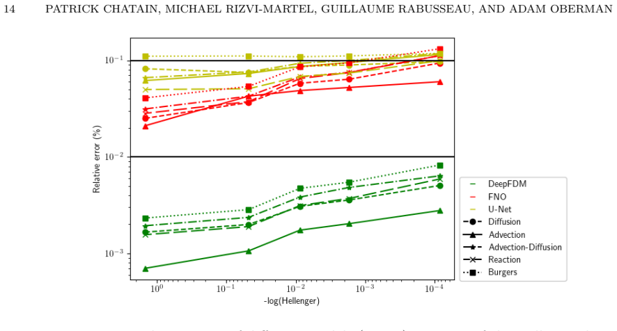
DeepFDM treats the forward pass of a neural network as a stable explicit finite-difference solve of the parametric family ∂tu = a0 + a1u + a2·∇u + a3Δu + b1u(1−u) + b2u∇u. Each convolution layer uses fixed difference stencils, such as [1,−2,1] for the Laplacian, and the learned grid functions Ai and Bj are the PDE coefficients, mapped through a scaled sigmoid so they stay inside the CFL stability region for the chosen time step and grid. Because a forward pass is a convergent first-order numerical solve with grid error O(h), the paper proves in Theorem 1 that training is a vector regression problem with noise shrinking at the grid resolution. Empirically, on in-distribution and out-of-distribution benchmarks quantified by Hellinger distance, DeepFDM's normalized MSE is 0.0007–0.0045 versus 0.025–0.04 for FNO, and its recovered coefficient fields match the ground truth. The paper also traces FNO's degradation on variable coefficients to its translation-invariant Green's-function assumption.
Load-bearing premise
The load-bearing premise is that the data-generation equations lie inside DeepFDM's fixed parametric family of scalar time-dependent PDEs, with coefficients bounded by the CFL stability condition and with boundary conditions that match the finite-difference stencil; if any of those fail, DeepFDM cannot represent the problem and its reported advantages disappear.
Editorial extensions
If this is right
- For scalar time-dependent PDEs whose form is known or contained in this parametric family, a trained DeepFDM is an order of magnitude more accurate than FNO, U-Net, and ResNet on the tested benchmarks, including under distribution shift.
- The 10–20x reduction in training epochs and 5–50x reduction in parameters means coefficient-identification problems of this type can be solved on modest compute budgets.
- Recovered coefficient fields let practitioners read off the spatially varying parameters of the PDE directly, rather than treating the solver as a black box.
- FNO's error grows with coefficient variance because its Fourier-space Green's-function assumption is translation invariant; DeepFDM's error stays nearly flat, so the advantage widens precisely when coefficients vary.
- Because the architecture is a convergent finite-difference scheme by construction, increasing resolution improves solution quality consistently, and out-of-distribution solutions follow the underlying PDE rather than learned interpolation.
Reading between the lines
- The comparison is framed against general-purpose neural operator backbones; a likely implicit boundary is that specialized learned solvers with built-in PDE structure, or models trained with larger datasets and better priors, could narrow the gap.
- The parametric-regression theorem suggests the method's advantage is really about statistical efficiency: when the hypothesis class contains the true solution operator, sample complexity and generalization follow from classical regression, so the natural extension is to nonlinear PDEs with known form but unknown terms.
- A testable extension is to move beyond scalar equations to systems and to other boundary conditions; because DeepFDM's stencils and CFL bounds are fixed, those changes require re-engineering, and a fair extended benchmark would measure how much accuracy is lost when the PDE family is widened without architectural changes.
- The Hellinger-distance shift measure could be reused by other PDE learning papers as a standardized OOD metric, but it only captures shifts in the initial-condition distribution, not shifts in the PDE family or boundary conditions.
Editorial analysis
A structured set of objections, weighed in public.
Referee Report
Summary. The paper introduces DeepFDM, a differentiable finite-difference model whose trainable weights are coefficient fields in a parametric family of scalar time-dependent PDEs. Training is framed as a vector regression problem (Theorem 1). The paper reports 10-40x lower normalized MSE than FNO, U-Net, and ResNet on five PDEs, with fewer training epochs and parameters, and demonstrates coefficient recovery. It also proposes the Hellinger distance as an OOD shift measure. The conclusion is that numerical PDE solvers outperform neural PDE solvers.
Significance. The contribution is valuable as a transparent, interpretable baseline for parametric inverse problems and as a reminder that neural operator benchmarks should include classical numerical solvers. Strengths include the interpretable parameterization with stability constraints, the simple regression perspective, reproducible code, and coefficient recovery. However, the empirical support for the headline claim is incomplete: the OOD test data are generated by DeepFDM's own forward solver, no error bars are reported, and the tested PDE family is narrow. The paper's significance would be substantially improved by an independent reference solver and a narrower, more precise title.
major comments (4)
- [§3.1, Eq. (4), Table 1] Section 3.1 states that additional data 'are generated by solving the numerical PDE solver (4), on a higher resolution grid, and then coarsen.' Equation (4) is exactly DeepFDM's forward operator NumSolve(U0; A(X)). Thus the OOD test set used for Table 1 is produced by the same finite-difference scheme, the same PDE family, and the same coefficient bounds that DeepFDM implements, while FNO, U-Net, and ResNet do not share the generator. The reported 30-40x OOD advantage is therefore evidence that DeepFDM can fit data generated by its own forward pass, not a general comparison of numerical and neural PDE solvers. Independent data from a different discretization or an analytic solution, and explicit boundary conditions, are needed.
- [§5, Theorem 1, §3.1] The proof of Theorem 1 defines epsilon_i = NumSolve(U0; A) - PDESolve(u0, a)(X) and obtains norm O(h) from standard error estimates. But for data generated as in Section 3.1, Ui is itself a NumSolve output (run at higher resolution and coarsened), so Ui - NumSolve(U0; A*) is a difference between two nested instances of the same solver, not an independent discretization error against the true PDE solution. The O(h) bound is therefore not established for the actual training pipeline, and the favorable bias of DeepFDM is built into the data-generation process. Using an independent high-order reference solver, or at least reporting the difference between the two discretizations, would resolve this concern.
- [§8, Tables 1-2, §1.2] The central claim is broader than the evidence. Table 2 reports only averages over three runs, with no standard deviations or per-run values, and Table 1 aggregates over just five scalar, time-dependent PDEs with known form and matching boundary settings. Moreover, the data-generating distribution in Section 1.2 is the same parametric family that DeepFDM is designed to invert. The title 'Numerical PDE solvers outperform neural PDE solvers' is not supported as a general statement; please restrict the claim to the tested family and add error bars and out-of-family tests.
- [§6.2, Eq. (8)] Equation (8) uses a plain sigmoid sigma(A_i) on the coefficient fields, so the effective diffusion coefficient is c_t sigma(A_i)/c_x^2, whose upper bound is c_t/c_x^2, not C_a = c_x^2/(2D c_t) as stated in (CFL). Section 6.2 says the parameters are scaled by C_a * sigma(theta) before multiplication with the Laplacian kernel, but that scaling is absent from Eq. (8). As written, the update rule does not enforce the CFL constraint, so the claim that DeepFDM is stable 'by design' is not supported by the equation. Please correct Eq. (8) or clarify the scaling used in the implementation.
minor comments (3)
- [Abstract, §7] The abstract says OOD is quantified by the Hellinger distance between 'coefficient priors', but Section 7 defines the Hellinger distance between distributions of Fourier coefficients of the initial conditions, not between distributions of the PDE coefficients a(x), b(x). Please reword to state that the shift is in the initial-condition distribution.
- [Table 3, Table 1, Abstract] The parameter-count claims are not consistently stated: Table 3 shows that DeepFDM's parameter count grows with grid resolution while FNO and U-Net counts are fixed, and at the 4096-point resolution Table 1 gives a 9x ratio to FNO, not the abstract's '5-50x'. ResNet actually has fewer parameters than DeepFDM at that resolution. Please specify the comparison baseline and resolution for every parameter-efficiency claim.
- [§9.4] The explanation that FNO's error growth with coefficient variance is due to the translation-invariance assumption is plausible but is not tested directly; a control experiment with translation-invariant coefficients would strengthen the causal claim.
Circularity Check
Benchmark data are generated by DeepFDM's own forward operator (Eq. 4), so the reported OOD and in-distribution accuracy advantages are partly built into the experimental design.
-
self definitional
[Section 3.1 ('Data generation for PDE solutions'), Eq. (4); see also Section 6.4 and Section 7]
"However, we also generate data by solving the numerical PDE solver (4), on a higher resolution grid, and then coarsen (upsample), onto the desired grid. Since the solver is accurate, it approximates the PDE solution."
Eq. (4) defines DeepFDM's forward pass as NumSolve(U0; A(X)), and Section 6.4 states the model 'corresponds by design' to a stable finite difference method. The target data are therefore generated by the same forward-Euler, CFL-bounded finite-difference scheme that DeepFDM implements (Section 7 states the generator 'uses the forward Euler method'). DeepFDM is thus trained and evaluated on outputs of its own forward operator, while FNO, U-Net, and ResNet are not given the generating discretization. This makes the comparison lopsided: the learned numerical solver is asked to invert the exact scheme that produced the data.
-
self definitional
[Section 8.1 ('Out-of-distribution data') and Table 1; see also Section 7]
"We generate PDE solution data by choosing families of orthogonal functions with random coefficients for the initial conditions, and passing these functions through a high accuracy numerical PDE solver."
The OOD test sets are produced by a numerical PDE solver of the same parametric family and the same forward-Euler discretization family that DeepFDM uses (Section 7: 'The PDE solver uses the forward Euler method... This solver can be used to generate high resolution PDE solutions'). The reported 30X-40X OOD improvement in Table 1 therefore measures how well DeepFDM extrapolates within its own discretization class, not how numerical solvers generally outperform neural operators on arbitrary data. The neural baselines do not share the generating scheme, so the OOD advantage is in part an artifact of testing a model on data generated by the model's own forward pass.
full rationale
The central empirical claim that DeepFDM outperforms neural PDE solvers rests on a benchmark whose data are generated by DeepFDM's own finite-difference solver: Section 3.1 says data are produced by 'the numerical PDE solver (4)', and Eq. (4) is exactly DeepFDM's forward operator NumSolve(U0; A(X)). The OOD data used for the headline improvement are also generated by a 'numerical PDE solver' of the same forward-Euler family (Sections 7 and 8.1). This makes the conclusion partially tautological: the model is tested on data from its own discretization, while the neural baselines must learn the map from generic data. The Theorem 1 noise model assumes Ui are evaluations of the true PDE solution, but for the generated data Ui are coarsened outputs of the same scheme, so the favorable O(h) residual assumption is not satisfied for that portion of the benchmark. There is no load-bearing self-citation chain: [Obe06] is an external published stability theory result, and [LT09] is a standard numerical-analysis reference; these do not independently raise the score. The in-distribution data sourced from [LSZ+22] provide some external content, and coefficient identification within the true family is a legitimate inverse problem, so the circularity is partial rather than total. The paper also leaves boundary conditions unspecified, which further limits external validity but is a correctness concern rather than circularity. Overall, score 6: one or more 'predictions' (especially OOD) reduce by construction to the model's own generating operator.
Assumptions & free parameters
free parameters (2)
- PDE coefficient fields a_i(x), b_j(x) =
learned from data; values depend on benchmark
- time step c_t and grid spacing c_x =
not fit; chosen to satisfy CFL (Ca = c_x^2/(2D c_t))
assumptions (4)
- standard math CFL stability condition 0 <= a(x) <= c_x^2/(2D c_t) for forward Euler discretization
- standard math First-order convergence of the finite difference scheme used in NumSolve
- domain assumption Well-posedness of the PDE family (Eq. PDE) for all admissible bounded coefficients
- domain assumption The data-generating distribution follows the same parametric family and coefficient bounds as DeepFDM
Cite this review
Pith. "Pith review of Numerical PDE solvers outperform neural PDE solvers." pith.science (2026). https://pith.science/paper/MENK2YFC
@misc{pith2026250721269,
  author       = {Pith},
  title        = {Pith review of: Numerical PDE solvers outperform neural PDE solvers},
  year         = {2026},
  howpublished = {\url{https://pith.science/paper/MENK2YFC}},
  note         = {Machine review of arXiv:2507.21269}
}
read the original abstract
We present DeepFDM, a differentiable finite-difference framework for learning spatially varying coefficients in time-dependent partial differential equations (PDEs). By embedding a classical forward-Euler discretization into a convolutional architecture, DeepFDM enforces stability and first-order convergence via CFL-compliant coefficient parameterizations. Model weights correspond directly to PDE coefficients, yielding an interpretable inverse-problem formulation. We evaluate DeepFDM on a benchmark suite of scalar PDEs: advection, diffusion, advection-diffusion, reaction-diffusion and inhomogeneous Burgers' equations-in one, two and three spatial dimensions. In both in-distribution and out-of-distribution tests (quantified by the Hellinger distance between coefficient priors), DeepFDM attains normalized mean-squared errors one to two orders of magnitude smaller than Fourier Neural Operators, U-Nets and ResNets; requires 10-20X fewer training epochs; and uses 5-50X fewer parameters. Moreover, recovered coefficient fields accurately match ground-truth parameters. These results establish DeepFDM as a robust, efficient, and transparent baseline for data-driven solution and identification of parametric PDEs.
Figures


Figures from the paper (4 more)



Forward citations
Cited by 1 Pith paper
-
Identifiability Limits of Physics-Informed Inference for Spatial Stochastic Dynamics from Static Snapshots
Structural identifiability analysis shows point sources restore identifiability for inferring spatial stochastic dynamics parameters from static snapshots, unlike distributed sources, with limits depending on modeling...
Reference graph
Works this paper leans on
-
[8]
On the convergence and generalization of physics informed neural networks
[SDK20] Yeonjong Shin, Jerome Darbon, and George Em Karniadakis. On the convergence and generalization of physics informed neural networks. arXiv e-prints , pages arXiv–2004,
work page 2004
-
[9]
Pdebench: An extensive benchmark for scientific machine learning
[TPL+22] Makoto Takamoto, Timothy Praditia, Raphael Leiteritz, Daniel MacKinlay, Francesco Alesiani, Dirk Pfl¨ uger, and Mathias Niepert. Pdebench: An extensive benchmark for scientific machine learning. In Sanmi Koyejo, S. Mohamed, A. Agarwal, Danielle Belgrave, K. Cho, and A. Oh, editors, Advances in Neural Information Processing Systems 35: Annual Conf...
work page 2022
-
[11]
Solver-in-the- loop: Learning from differentiable physics to interact with iterative pde-solvers
[UBF+20] Kiwon Um, Robert Brand, Yun (Raymond) Fei, Philipp Holl, and Nils Thuerey. Solver-in-the- loop: Learning from differentiable physics to interact with iterative pde-solvers. In Hugo Larochelle, Marc’Aurelio Ranzato, Raia Hadsell, Maria-Florina Balcan, and Hsuan-Tien Lin, editors, Advances in Neural Information Processing Systems 33: Annual Confere...
work page 2020
-
[12]
Climode: Climate and weather forecasting with physics-informed neural odes
[VHG24] Yogesh Verma, Markus Heinonen, and Vikas Garg. Climode: Climate and weather forecasting with physics-informed neural odes. In The Twelfth International Conference on Learning Representations, ICLR 2024, Vienna, Austria, May 7-11, 2024 . OpenReview.net,
work page 2024
- [14]
-
[2006]
[JYHL24] A. Jiao, Q. Yan, J. Harlim, and L. Lu. Solving forward and inverse pde problems on unknown manifolds via physics-informed neural operators. arXiv preprint arXiv:2407.05477 ,
-
[2012]
Accessed: 2024-09-26. [LSZ+22] Xin-Yang Liu, Hao Sun, Min Zhu, Lu Lu, and Jian-Xun Wang. Predicting parametric spatiotemporal dynamics by multi-resolution pde structure-preserved deep learning. arXiv preprint arXiv:2205.03990 ,
work page Pith review arXiv 2024
-
[2017]
U-net: Convolutional networks for biomedical image segmentation
[RFB15] Olaf Ronneberger, Philipp Fischer, and Thomas Brox. U-net: Convolutional networks for biomedical image segmentation. In Medical image computing and computer-assisted intervention–MICCAI 2015: 18th international conference, Munich, Germany, October 5-9, 2015, proceedings, part III 18 , pages 234–241. Springer,
work page 2015
Show all 14 references
-
[2019]
Fourier neural operator for parametric partial differential equations
[LKA+20a] Zongyi Li, Nikola Kovachki, Kamyar Azizzadenesheli, Burigede Liu, Kaushik Bhattacharya, Andrew Stuart, and Anima Anandkumar. Fourier neural operator for parametric partial differential equations. arXiv preprint arXiv:2010.08895 , 10
2010 arXiv
-
[2020]
Neural operator: Graph kernel network for partial differential equations
[LKA+20b] Zongyi Li, Nikola Kovachki, Kamyar Azizzadenesheli, Burigede Liu, Kaushik Bhattacharya, Andrew Stu- art, and Anima Anandkumar. Neural operator: Graph kernel network for partial differential equations. arXiv preprint arXiv:2003.03485 , 03
2003 arXiv
-
[2021]
Deeponet: Learning nonlinear operators for identi- fying differential equations based on the universal approximation theorem of operators
[LJK19] Lu Lu, Pengzhan Jin, and George Em Karniadakis. Deeponet: Learning nonlinear operators for identi- fying differential equations based on the universal approximation theorem of operators. arXiv preprint arXiv:1910.03193,
1910 arXiv
-
[2022]
Neural stochastic differential equations: Deep latent gaussian models in the diffusion limit
[TR19] Belinda Tzen and Maxim Raginsky. Neural stochastic differential equations: Deep latent gaussian models in the diffusion limit. arXiv preprint arXiv:1905.09883 ,
1905 arXiv
-
[2023]
[CORJO23] L
Accessed: 2024- 09-26. [CORJO23] L. Cao, T. O’Leary-Roseberry, P.K. Jha, and J.T. Oden. Residual-based error correction for neural operator accelerated infinite-dimensional bayesian inverse problems. Journal of Computational Physics ,
2024
-
[2024]
[ZL W22] Qingqing Zhao, David B
Version 1.0. [ZL W22] Qingqing Zhao, David B. Lindell, and Gordon Wetzstein. Learning to solve pde-constrained inverse problems with graph networks. In Kamalika Chaudhuri, Stefanie Jegelka, Le Song, Csaba Szepesv´ ari, Gang Niu, and Sivan Sabato, editors, International Confere...
2022
Reviewed August 6, 2026 · model on record in the stance chip above.
Discussion (0). Sign in to comment.