REVIEW 3 major objections 6 minor 39 references
Hierarchical Stochastic Differential Equation Models for Latent Manifold Learning in Neural Time Series
T0 review · 3 major / 6 minor · reviewed 2026-08-06 · deepseek-v4-flash
Pith's one-line read Sparse inducing points, joined by Brownian-bridge SDEs, let a hierarchical model uniformly approximate any continuous trajectory while keeping inference linear in time.
desk verdict New hierarchical SDE architecture worth knowing, but the discrete-time inference in Eq. (18) uses the wrong noise scaling, so the reported experiments are for a different, nearly deterministic process. read the letter →
The pith
A machine-rendered reading of the paper's core claim, the machinery that carries it, and where it could break.
The reading
What carries the argument
The load-bearing object is the hierarchical pair of SDEs. Inducing points $(\tau_i, m_i)$, drawn from a marked point process with Gamma waiting times and Gaussian marks, define a Brownian bridge process $X_t$—an SDE pinned to reach each mark at its time—whose path then serves as the drift of a second SDE $Y_t$; observations are a noisy linear projection of $Y_t$. The renewal-process simplification (waiting times and marks independent of history) breaks the non-Markovian dependence and makes sequential Monte Carlo inference possible. The universal approximation result rests on the density of piecewise-linear interpolants of uniformly spaced samples, with the bridge noise concentrated by Chebyshev's inequality.
What would settle it
Simulate a continuous $f$ with a sharp localized feature, generate observations from the true model with known inducing points, run the SMC inference at increasing particle counts, and measure $\sup_t |\mathbb{E}[Y_t] - \int_0^t f(s)\,ds|$; if the error does not shrink toward zero as $N$ grows—or if the inferred waiting times stay long near the sharp feature—the practical claim of adaptive, linear-cost universal approximation is contradicted.
Extended reading notes
Core claim
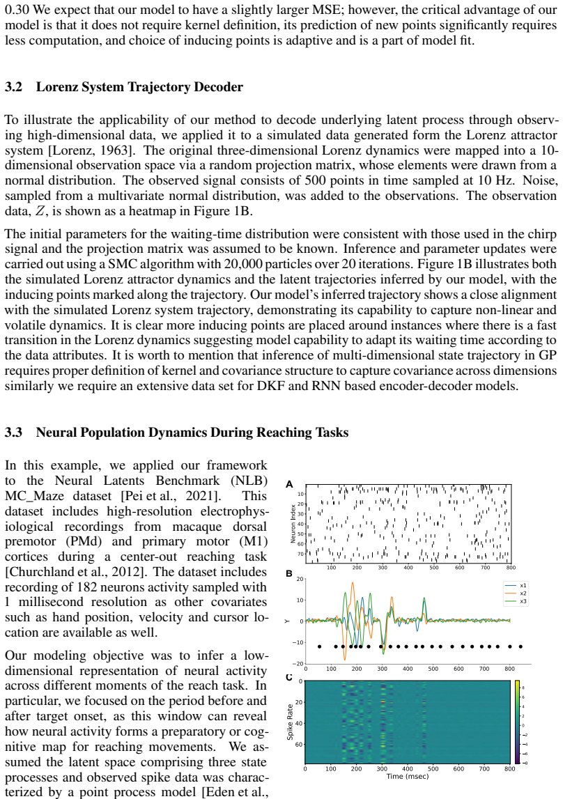
The paper's central claim is that a cascade of two SDEs—an inner Brownian bridge constrained to pass through sampled marks at sampled times, and an outer process whose drift is the inner path—is expressive enough to model any continuous low-dimensional signal while remaining tractable. The formal statement is a universal approximation theorem: for any continuous $f$ and any $\varepsilon > 0$, there exists a choice of inducing points such that $\mathbb{E}[Y_t]$ uniformly approximates $g(t) = \int_0^t f(s)\,ds$ within $\varepsilon$. The authors also claim that the discretized model can be trained and inferred with a custom particle filter whose cost per iteration is $O(P\cdot N)$, avoiding the cubic cost of Gaussian process inversion, and that the inducing points adapt to the data's temporal structure. They demonstrate the framework on synthetic chirp and Lorenz data and on neural population recordings, where the inferred latent trajectory changes around target onset, consistent with preparatory motor activity.
Load-bearing premise
The load-bearing premise is that waiting times between inducing points and their mark values can be treated as independent of each other and of past events (Eq. 2); if that independence fails to hold for a given dynamic, the model cannot adapt its inducing points to the data's temporal scales, as the authors acknowledge.
Editorial extensions
If this is right
- Inference cost scales as $O(P\cdot N)$ per SMC iteration, so long, high-resolution neural time series become feasible where Gaussian-process models hit $O(N^3)$.
- As the number of inducing points grows, the expected latent process can uniformly approximate the integral of any continuous function, so the model's expressiveness is not limited by a fixed parametric form.
- Inducing points are inferred from data and concentrate where dynamics change rapidly—for example, around fast Lorenz transitions—giving an interpretable summary of where the manifold is complex.
- The same latent process can be paired with point-process observation models, as in the reaching-task analysis, making it applicable to spike-train recordings rather than only continuous observations.
- Because the model needs no pre-specified kernel, it offers a nonparametric alternative to GP-based latent dynamic models for exploratory neural data analysis.
Reading between the lines
- The universal approximation theorem guarantees existence of good inducing points, not that the SMC inference will find them; a direct test of posterior concentration as $N$ grows would separate expressiveness from recoverability.
- The independence assumption in Eq. (2) forces waiting times to be drawn afresh regardless of how fast the signal is changing, so the model may systematically under-sample sharp transitions; a history-dependent or repulsive prior, which the authors mention, would be a natural extension to test.
- The linear-cost claim depends on the number of particles $P$ staying fixed; comparing effective sample size and accuracy at fixed compute against Kalman-filter hybrids could show whether the SMC overhead is actually necessary.
- Applied to neural decoding, the model's inferred $Y_t$ could be used as a real-time readout of preparatory dynamics; this is a testable extension the paper leaves open.
Editorial analysis
A structured set of objections, weighed in public.
Referee Report
Summary. The paper introduces a hierarchical stochastic differential equation model for latent manifold learning in neural time series. Inducing points, defined as time-mark pairs from a marked point process, parameterize Brownian-bridge SDEs whose expectation defines the drift of a second SDE layer; observations are noisy linear projections of the latent process. The authors prove a universal approximation property for the expected latent process, derive an SMC-based EM inference procedure claimed to scale linearly with sequence length, and present experiments on a chirp signal, a projected Lorenz system, and the NLB MC_Maze neural dataset. The central inference pipeline, however, is built on a discrete-time transition that does not correctly discretize the proposed SDE.
Significance. The modeling idea is attractive: a sparse, adaptive set of inducing points connected by Brownian bridges gives an interpretable, nonparametric latent dynamical model that avoids kernel choices and cubic GP scaling. The claimed O(P·N) inference cost and the universal approximation property are, if correct, useful contributions for neural time-series analysis. The paper also deserves credit for explicitly acknowledging the limitations of the independence assumption on waiting times and marks. However, the current manuscript is not reliable in its reported form because the discretization used in inference does not match the continuous SDE, so the empirical validations do not yet support the central claim that the proposed hierarchical SDE can be trained and inferred successfully.
major comments (3)
- [A.3, Eq. (18)] The discrete-time transition in Eq. (18) is not a valid Euler-Maruyama discretization of the SDE in Eqs. (3)-(4). For an Ito SDE dX_t = mu_t dt + sigma_t dW_t, the increment over a step of length dt is mu_t dt + sigma_t dW_t with dW_t ~ N(0, dt); hence the diffusion term must carry a factor sqrt(dt), not dt. As written, the variance of the X-increment is O(dt^2) rather than O(dt), so in the limit dt -> 0 the process converges to the deterministic ODE dX_t/dt = (m_{i+1} - X_t)/(t_{i+1} - t). Because Eq. (18) supplies the transition density p(X_k | tau, m) used in the importance weights of Algorithms 1 and 2, all reported posteriors over inducing points and latent trajectories are computed for a different, effectively noise-free process than the hierarchical SDE defined in Section 2.1. This is a load-bearing error in the inference pipeline and must be corrected (the sqrt(dt) factor) and the experiments rerun.
- [Section 2.1, Eq. (2); Section 4] The renewal assumption p(tau_i) p(m_i) in Eq. (2) is load-bearing: it is what allows the non-Markovian X process to be treated as Markovian in Algorithm 1 by conditioning on the next event time and mark. The authors acknowledge in Section 4 that this 'may reduce its ability to adjust inducing points to capture changes in data happening at different temporal scales.' This limitation is not merely cosmetic: because tau_i and m_i are generated independently of the data, the generative model has no mechanism for placing more inducing points where the dynamics are fast; any such adaptation in Figures 1B and 2 must come entirely from posterior reweighting. The paper should temper the claims of adaptive inducing-point placement or provide a quantitative comparison of posterior waiting times against data-driven event times.
- [Sections 3.1, 3.2, and 4] The diffusion parameters sigma_x and sigma_y and observation noise variance R are set by hand (e.g., sigma_x = 10^{-1}, sigma_y = 10^{-4} in Section 3.1; see also Section 4, where the authors state 'we adjust their values by checking different values for both'), yet the model's behavior is strongly controlled by these choices: sigma_x sets the flexibility of the interpolation paths and sigma_y controls how much observation information propagates back to X. The paper reports no sensitivity analysis or posterior uncertainty for these parameters. Since the central empirical claims are qualitative, the authors should at least show that the reported latent trajectories and inducing-point placements are stable across reasonable ranges of these parameters.
minor comments (6)
- [Section 2.2.1] The reference to Shannon's sampling theorem is misleading: the proof uses piecewise linear interpolation and density in C([0,T]), not bandlimited sampling; the connection to Shannon should be removed or clarified.
- [Section 2.2.1, proof] Chebyshev's inequality bounds the probability that a single time point deviates from its mean; the text writes 'Y_t concentrates around E[Y_t]' but the uniform-in-t statement used later requires a union bound or a modulus-of-continuity argument. This does not affect the main approximation claim, but the proof is slightly imprecise.
- [Algorithm 1, line 10] Sampling new tau and m from the prior with no data-dependent proposal is a weak proposal and may cause weight degeneracy; the paper does not report effective sample size (ESS), which would help assess the reliability of the SMC results.
- [Section 3.1] The comparison with the GP reports MSE values 0.22 and 0.30 without error bars or multiple restarts; the sentence 'We expect our model to have a slightly larger MSE' is not a substitute for a statistical comparison.
- [Section 3.2] The claim that 'more inducing points are placed around instances where there is a fast transition' is not quantified; a scatter of inferred tau_i against local |dZ/dt| or a similar diagnostic would strengthen the claim.
- [Throughout] There are several typographical errors (e.g., 'ne ural' in the abstract, 'Y ousefi' in the author list) and inconsistent notation (e.g., p used for both densities and probabilities in Eq. (2)); a careful proofreading pass is needed.
Circularity Check
No circular derivation: the universal approximation claim is an external density result, and the only self-citation is non-load-bearing.
full rationale
The paper's central theoretical claim, the universal approximation theorem in Section 2.2.1, is not circular. With zero diffusion, the Brownian bridge SDE in Eqs. (3)-(4) solves to exactly the piecewise linear interpolant between inducing points, so the proof's use of piecewise linear interpolation is the model itself evaluated in the deterministic limit; the claim then reduces to the standard density of piecewise-linear interpolants in C([0,T]) and the continuity of integration, both external mathematical facts. The theorem is not used to fit parameters or to define outputs in terms of observed targets. The only author self-citation, Ziaei et al. 2024, appears in the related-work list as an example of an existing latent-variable decoder and is not load-bearing for the derivation, the SMC algorithm, or the universal approximation proof. The empirical evaluations use external benchmark data (Lorenz system, NLB MC_Maze), so the conclusions are not derived from the model's own fitted quantities by construction. The manuscript's Appendix A.3, Eq. (18), does contain a potential discretization inconsistency—the diffusion term scales as Δt rather than √Δt—but that is a correctness/internal-consistency concern about whether the implemented inference matches the stated SDE, not a circularity in which a prediction reduces to its input. Manual choices of noise variances and the acknowledged independence assumption in Section 4 are modeling limitations, not circular steps. Accordingly, no circular steps are identified and the score is 0.
Assumptions & free parameters
free parameters (5)
- σx (diffusion of X process) =
set manually (e.g., 1e-1 in chirp example)
- σy (diffusion of Y process) =
set manually (e.g., 1e-4 in chirp example)
- Observation noise covariance R =
assumed known in chirp and Lorenz examples
- Latent dimensionality D =
3 in neural example
- Gamma shape α and rate λ for waiting times =
initial mean 40 s, std 8.94 in chirp; updated in M-step
assumptions (6)
- domain assumption Manifold hypothesis: high-dimensional neural time series lie on a low-dimensional manifold
- domain assumption Sparse trajectory samples (inducing points) are sufficient to reconstruct the manifold trajectory
- domain assumption Waiting times and marks are independent and identically distributed, independent of history
- domain assumption Linear projection between latent states and observations
- standard math Density of piecewise linear functions in C([0,T])
- standard math Existence and uniqueness of SDE solutions (Brownian bridge and integrated process)
Cite this review
Pith. "Pith review of Hierarchical Stochastic Differential Equation Models for Latent Manifold Learning in Neural Time Series." pith.science (2026). https://pith.science/paper/UFNMLIGR
@misc{pith2026250721531,
  author       = {Pith},
  title        = {Pith review of: Hierarchical Stochastic Differential Equation Models for Latent Manifold Learning in Neural Time Series},
  year         = {2026},
  howpublished = {\url{https://pith.science/paper/UFNMLIGR}},
  note         = {Machine review of arXiv:2507.21531}
}
read the original abstract
The manifold hypothesis suggests that high-dimensional neural time series lie on a low-dimensional manifold shaped by simpler underlying dynamics. To uncover this structure, latent dynamical variable models such as state-space models, recurrent neural networks, neural ordinary differential equations, and Gaussian Process Latent Variable Models are widely used. We propose a novel hierarchical stochastic differential equation (SDE) model that balances computational efficiency and interpretability, addressing key limitations of existing methods. Our model assumes the trajectory of a manifold can be reconstructed from a sparse set of samples from the manifold trajectory. The latent space is modeled using Brownian bridge SDEs, with points - specified in both time and value - sampled from a multivariate marked point process. These Brownian bridges define the drift of a second set of SDEs, which are then mapped to the observed data. This yields a continuous, differentiable latent process capable of modeling arbitrarily complex time series as the number of manifold points increases. We derive training and inference procedures and show that the computational cost of inference scales linearly with the length of the observation data. We then validate our model on both synthetic data and neural recordings to demonstrate that it accurately recovers the underlying manifold structure and scales effectively with data dimensionality.
Figures


Reference graph
Works this paper leans on
-
[1]
G. Bondanelli, T. Deneux, B. Bathellier, and S. Ostojic. Network dynamics underlying off responses in the auditory cortex. Elife, 10: 0 e53151, 2021
work page 2021
-
[2]
E. N. Brown and R. E. Kass. Estimating a state-space model from point process observations. Unpublished Manuscript, 2018
work page 2018
-
[3]
F. P. Casale, A. V. Dalca, L. Saglietti, J. Listgarten, and N. Fusi. Gaussian process prior variational autoencoders. 31, 2018
work page 2018
- [4]
-
[5]
R. T. Q. Chen, Y. Rubanova, J. Bettencourt, and D. Duvenaud. Neural ordinary differential equations. 31, 2018
work page 2018
-
[6]
M. M. Churchland, J. P. Cunningham, M. T. Kaufman, S. I. Ryu, and K. V. Shenoy. Neural population dynamics during reaching. Nature, 487 0 (7405): 0 51--56, 2012
work page 2012
-
[7]
J. P. Cunningham and B. M. Yu. Dimensionality reduction for large-scale neural recordings. Nature neuroscience, 17 0 (11): 0 1500--1509, 2014
work page 2014
-
[8]
D. J. Daley and D. Vere-Jones. An introduction to the theory of point processes: volume I: elementary theory and methods. Springer Science & Business Media, 2006
work page 2006
Show all 39 references
-
[9]
Doucet, N
A. Doucet, N. de Freitas, and N. Gordon. Sequential Monte Carlo Methods in Practice. Springer, New York, 2001
2001
-
[10]
U. T. Eden, L. M. Frank, R. Barbieri, V. Solo, and E. N. Brown. Dynamic analysis of neural encoding by point process adaptive filtering. Neural Computation, 16 0 (5): 0 971--998, 2004
2004
-
[11]
Eleftheriadis, T
S. Eleftheriadis, T. Nicholson, M. Deisenroth, and J. Hensman. Identification of gaussian process state space models. Advances in neural information processing systems, 30, 2017
2017
-
[12]
E. Fox, E. Sudderth, M. Jordan, and A. Willsky. Nonparametric bayesian learning of switching linear dynamical systems. In D. Koller, D. Schuurmans, Y. Bengio, and L. Bottou, editors, Advances in Neural Information Processing Systems, volume 21. Curran Associates, Inc., 2008
2008
-
[13]
Ghahramani and G
Z. Ghahramani and G. E. Hinton. Variational learning for switching state-space models. Neural Computation, 12 0 (4): 0 831--864, 2000. doi:10.1162/089976600300015619
-
[14]
Girin, S
L. Girin, S. Leglaive, X. Bie, J. Diard, T. Hueber, and X. Alameda-Pineda. Dynamical variational autoencoders: A comprehensive review. arXiv preprint arXiv:2008.12595, 2020
2008 arXiv
-
[15]
Glorot and Y
X. Glorot and Y. Bengio. Understanding the difficulty of training deep feedforward neural networks. In Proceedings of the Thirteenth International Conference on Artificial Intelligence and Statistics (AISTATS), pages 249--256. PMLR, 2010
2010
-
[16]
Gonzalez-Castillo, I
J. Gonzalez-Castillo, I. S. Fernandez, K. C. Lam, D. A. Handwerker, F. Pereira, and P. A. Bandettini. Manifold learning for fmri time-varying functional connectivity. Frontiers in Human Neuroscience, 17: 0 1134012, 2023
2023
-
[17]
Gosztolai, R
A. Gosztolai, R. L. Peach, A. Arnaudon, M. Barahona, and P. Vandergheynst. Interpretable statistical representations of neural population dynamics and geometry. arXiv preprint, 2023
2023
-
[18]
W. K. Hastings. Monte carlo sampling methods using markov chains and their applications. Biometrika, 57 0 (1): 0 97--109, 1970
1970
-
[19]
Jacobsen
M. Jacobsen. Point Process Theory and Applications: Marked Point and Piecewise Deterministic Processes. Birkhäuser, Boston, 2006
2006
-
[20]
R. G. Krishnan, U. Shalit, and D. Sontag. Deep kalman filters, 2015 a
2015
-
[21]
R. G. Krishnan, U. Shalit, and D. Sontag. Deep kalman filters. arXiv preprint arXiv:1511.05121, 2015 b
2015 arXiv
-
[22]
Kwon, H.-S
J. Kwon, H.-S. Oh, and Y. Lim. Dynamic principal component analysis with missing values. Journal of Applied Statistics, 47 0 (11): 0 1957--1969, 2020
1957
-
[23]
E. N. Lorenz. Deterministic nonperiodic flow. Journal of the Atmospheric Sciences, 20 0 (2): 0 130--141, 1963
1963
-
[24]
McInnes, J
L. McInnes, J. Healy, and J. Melville. Umap: Uniform manifold approximation and projection for dimension reduction. arXiv preprint arXiv:1802.03426, 2018
2018 arXiv
-
[25]
Oksendal
B. Oksendal. Stochastic differential equations: an introduction with applications. Springer Science & Business Media, 2013
2013
-
[26]
F. Pei, J. Ye, D. M. Zoltowski, A. Wu, R. H. Chowdhury, H. Sohn, J. E. O'Doherty, K. V. Shenoy, M. T. Kaufman, M. M. Churchland, M. Jazayeri, L. E. Miller, J. W. Pillow, I. M. Park, E. L. Dyer, and C. Pandarinath. Neural latents benchmark '21: Evaluating latent variable models...
2021
-
[27]
Petralia, V
F. Petralia, V. Rao, and D. Dunson. Repulsive mixtures. Advances in neural information processing systems, 25, 2012
2012
-
[28]
Pitman and M
J. Pitman and M. Yor. Brownian bridge and related stochastic processes. Probability Surveys, 1: 0 1--61, 1999
1999
-
[29]
S. S. Rangapuram, M. W. Seeger, J. Gasthaus, L. Stella, Y. Wang, and T. Januschowski. Deep state space models for time series forecasting. Advances in neural information processing systems, 31, 2018
2018
-
[30]
T. K. Rusch and D. Rus. Linear oscillatory state-space models. Proceedings of the International Conference on Learning Representations (ICLR), 2025
2025
-
[31]
S \"a rkk \"a and L
S. S \"a rkk \"a and L. Svensson. Bayesian filtering and smoothing, volume 17. Cambridge university press, 2023
2023
-
[32]
M. Seeger. Gaussian processes for machine learning. International journal of neural systems, 14 0 (02): 0 69--106, 2004
2004
-
[33]
C. E. Shannon. Communication in the presence of noise. Proceedings of the IRE, 37 0 (1): 0 10--21, 1949
1949
-
[34]
G. E. Uhlenbeck and L. S. Ornstein. On the theory of the brownian motion. Physical Review, 36 0 (5): 0 823--841, 1930
1930
-
[35]
Van der Maaten and G
L. Van der Maaten and G. Hinton. Visualizing data using t-sne. Journal of machine learning research, 9 0 (11), 2008
2008
-
[36]
J. Wang, A. Hertzmann, and D. J. Fleet. Gaussian process dynamical models. Advances in neural information processing systems, 18, 2005
2005
-
[37]
Whiteley, A
N. Whiteley, A. Gray, and P. Rubin-Delanchy. Statistical exploration of the manifold hypothesis, 2024
2024
-
[38]
Z. Xu, L. Zhang, and Y. Lu. Variational posterior approximation using stochastic gradient ascent for dirichlet process mixture models. Pattern Recognition, 110: 0 107637, 2021
2021
-
[39]
Ziaei, B
N. Ziaei, B. Nazari, U. T. Eden, A. Widge, and A. Yousefi. A bayesian gaussian process-based latent discriminative generative decoder (ldgd) model for high-dimensional data. IEEE Access, 2024
2024
Reviewed August 6, 2026 · model on record in the stance chip above.
Discussion (0). Sign in to comment.