REVIEW 4 major objections 6 minor 113 references
Non-periodic Fourier propagation algorithms for partial differential equations
T0 review · 4 major / 6 minor · reviewed 2026-08-06 · deepseek-v4-flash
Pith's one-line read Fourier solver reaches machine precision on non-periodic PDEs.
desk verdict Solid, honest numerical-methods paper: DST/DCT plus interaction picture is genuinely useful for non-periodic parabolic and stochastic PDEs, but the time-varying-boundary claim needs a stronger test and one formula has a dimensional slip. read the letter →
The pith
A machine-rendered reading of the paper's core claim, the machinery that carries it, and where it could break.
The reading
What carries the argument
The central object is the Fourier interaction picture (FIP): a split-step scheme in which the linear, constant-coefficient part of a PDE is advanced exactly through a spectral Green's function propagator $G(t,t')=\exp[(t-t')\mathcal{L}]$ that is diagonal in the DST/DCT basis, while the nonlinear, stochastic, or explicitly coordinate-dependent terms are integrated as an ordinary differential equation in the interaction picture. The discrete sine and cosine transforms are chosen according to the boundary type—DST-I for Dirichlet-Dirichlet, DCT-I for Neumann-Neumann, DST-II/III and DCT-II/III for mixed boundaries—and the derivative operator becomes exactly diagonal with eigenvalues proportional to $k_n^2$, where $k_n=(n-1)\pi/R$ or $(n-1/2)\pi/R$ depending on the transform. Inhomogeneous, time-dependent boundary values are handled by subtracting a smooth polynomial patch function that satisfies the boundary conditions and (for FIP) locally solves the PDE over a short time interval, after which the residual field obeys homogeneous boundary conditions. The whole scheme is a special case of the Galerkin approximation, as shown in the appendices, but one that keeps the uniformity of the spatial grid and the $N\ln N$ speed of fast transforms.
What would settle it
Run the FIP method on the 1D heat equation with a boundary value that changes rapidly on the time-step scale, e.g. $u(0,t)=\sin(\omega t)$ with $\omega \Delta t \gg 1$, and compare the RMS error against the analytic solution; if the error jumps to the level of the polynomial solvers (or worse), the claim that the method handles time-dependent Dirichlet and Neumann boundaries at machine precision fails.
Extended reading notes
Core claim
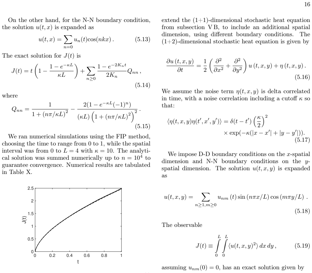
The central claim is that the interaction-picture extension of Fourier spectral methods, built on fast discrete sine and cosine transforms (DST/DCT) and a diagonal spectral propagator, is a competitive and often superior solver for parabolic PDEs and SPDEs with non-periodic boundaries. The paper demonstrates this by converting an inhomogeneous boundary-value problem into a homogeneous one through low-order polynomial patch functions, then treating the homogeneous part with the transform whose boundary type (Dirichlet or Neumann) matches the problem. For the linear heat equation, the FIP method yields errors at the level of machine precision for all four combinations of Dirichlet and Neumann boundary conditions, roughly $10^{12}$ times smaller than the compared Tau and Galerkin methods at identical step sizes. For nonlinear equations with localized peaks, the Peregrine wave and the breather of the nonlinear Schrödinger equation, the Fourier methods' errors are one to three orders of magnitude lower than the polynomial solvers, at comparable or lower computation time. For the stochastic heat equation, FIP achieves lower errors and runs several times faster than the Tau method, and the paper further shows that spatially filtered (correlated) noise is generated efficiently on the uniform grid, extending the method to one and two spatial dimensions.
Load-bearing premise
The whole scheme assumes that the boundary values change slowly enough over one time step that a simple polynomial patch function satisfies the PDE near the boundary; if boundary values vary rapidly or stochastically in time, the patch no longer solves the PDE and the claimed accuracy is not guaranteed.
Editorial extensions
If this is right
- For linear parabolic equations with constant coefficients and Dirichlet or Neumann boundaries, the FIP method achieves machine-precision accuracy with relatively large time steps (e.g., $\Delta t=0.1$ in the heat equation), eliminating the need for very small steps.
- For problems with rapid spatial variation—localized peaks, solitary waves, breathers—uniform-grid Fourier methods deliver errors one to three orders of magnitude below Chebyshev/Legendre Tau and Galerkin solvers at the same step sizes, and are generally faster.
- For stochastic PDEs with delta-correlated spatial noise, where the solution does not become smoother as the grid is refined, the FIP method retains its accuracy advantage over polynomial spectral methods, and the uniform grid makes generation of spatially correlated (filtered) noise straightforward.
- The methods extend to multiple space dimensions and to per-component, per-dimension mixtures of Dirichlet and Neumann boundary conditions, as demonstrated by the (1+2)-dimensional stochastic heat equation with filtered noise.
- At a fixed total resource (space steps times time steps), the FIP method attains lower minimum error than the Tau method with the same temporal order, although the Tau method has a better asymptotic spatial convergence rate for smooth solutions.
Reading between the lines
- The machine-precision result is for problems where the inhomogeneous part is exactly linear in the field and the patch is exactly time-independent; for genuinely nonlinear or stochastic boundary data, the method's accuracy will likely degrade to the time-integration order, so the practical regime of 'machine precision' should be read as limited to linear boundaries.
- Because the derivative matrix is diagonal in the DST/DCT basis, the method is naturally suited to stiffness-dominated problems (e.g., the biharmonic operator) where implicit or exact linear propagation avoids the von Neumann step restriction; testing fourth-order operators with FIP would be a direct extension.
- The uniform-grid property is also a bridge to deep-learning surrogates and neural operator methods for PDEs, which usually expect equispaced input; the paper notes this connection but does not exploit it.
- For stochastic problems, the method's advantage is likely to persist for any noise with a spatial spectrum that is not rapidly decaying, since the uniform grid resolves high-wavenumber noise efficiently; a testable prediction is that FIP remains superior for power-law correlated noise.
Editorial analysis
A structured set of objections, weighed in public.
Referee Report
Summary. The paper introduces two Fourier spectral algorithms, FSD and FIP, for parabolic PDEs and SPDEs with non-periodic boundary conditions on uniform grids. The spatial discretization uses discrete sine and cosine transforms selected according to the boundary type (D-D, D-N, N-D, N-N), and inhomogeneous boundary data are handled by adding polynomial patch functions. The methods are validated against analytical solutions for the 1D heat equation, the Peregrine soliton, a breather, a double simulton, and stochastic heat equations in one and two dimensions with delta-correlated and filtered noise. Comparisons are made with the Dedalus (Tau) and MATLAB pdepe (Galerkin) solvers, together with a fixed-resource complexity analysis. The central reported results are machine-precision accuracy of FIP for the linear heat equation, lower errors for localized nonlinear and stochastic problems, and speed advantages over the polynomial solvers, with the caveat that the Tau method is more accurate for a smooth simulton case.
Significance. If the claims hold, the paper provides a useful uniform-grid alternative to polynomial spectral methods for non-periodic parabolic problems, particularly for solutions with localized spatial structure or stochastic noise. Strengths include the use of exact analytical benchmark solutions, the absence of fitted parameters, the public-domain xSPDE4 implementation, and a balanced comparison that explicitly identifies a smooth-solution regime in which polynomial methods are superior. The interaction-picture linear propagator for the heat equation gives genuinely striking accuracy. However, the generality of the time-varying boundary condition treatment rests on an approximate patch construction that is not stress-tested, and a few printed formulas and claims need correction. These issues are fixable but currently prevent full confidence in the paper's broadest conclusions.
major comments (4)
- [III A, Eq. (3.15)] The Neumann-Neumann patch is dimensionally inconsistent. From Eq. (3.12), one has ∂t v = ε, while D₂∇²v = D₂(N_b−N_a)/(x_b−x_a). Enforcing ∂t v = D₂∇²v gives ε = D₂(N_b−N_a)/(x_b−x_a); the printed Eq. (3.15) contains an extra factor Δt, so the patch as written does not satisfy the local PDE except in the special case Δt = 1. If the implementation used the correct unprinted form, the text must be corrected; if not, the N-N time-dependent results are not produced by the stated algorithm.
- [III A and IV D] The treatment of time-dependent boundary conditions is only approximate, and the claim that the midpoint algorithm is exempt from order reduction is not tested. The D-D, D-N, and N-D patches in Eqs. (3.2), (3.5), and (3.8) are linear in x, so for time-dependent boundary values ∂t v is nonzero while the Laplacian term vanishes; the patch does not locally solve the heat equation. The paper acknowledges this with the sentence 'for simplicity we suppose that the boundary condition is approximately time-independent over a short time-interval,' but in Section IV D it then asserts that the order-reduction and spurious-boundary-layer issues of [81] 'are not observed when the midpoint algorithm is used.' No experiment with rapidly varying or stochastic boundary data is reported; all boundary data in Tables I-IV and V-XI are either zero or slowly varying relative to Δt. Since the abstract and conclusion claim time-varying Dirichlet/Neumann/Robin boundary conditions in general, this is a load-bearing gap. Please add a quantitative test with rapidly varying boundary data, or restrict the stated scope.
- [IV D, V, Conclusion] The fine-grid behavior of FIP is left as speculation. In Tables V and VI the FIP error scaling drops from quadratic to sublinear for fine grids, and the conclusion says this regime is 'presumably needing a momentum-space filter [93],' but no filter is implemented or tested. Since the complexity analysis and performance claims focus on exactly this regime, the reader cannot tell whether the behavior is a fundamental limitation or an easily fixed implementation detail. Either implement and test the filter, or clearly delimit the range of step sizes over which the method is recommended.
- [I (introduction)] The introduction states that 'our interaction picture algorithm has clear advantages over these' prior DST/DCT methods [24,25], but the paper neither compares with those algorithms nor identifies precisely what new capability the FIP formulation adds beyond them. Without such a comparison or at least a precise statement of the algorithmic difference, the claimed advantage is not supported by the evidence in the paper.
minor comments (6)
- [II F, Eq. (2.31)] In Eq. (2.31), 'Δ/2' should be 'Δt/2'.
- [II B and Conclusion] The conclusion mentions Robin boundary conditions, but the paper defines and implements only Dirichlet, Neumann, and periodic boundary conditions (Eqs. 2.7-2.9); please either implement Robin boundary conditions or remove the claim.
- [III B and experimental sections] The pseudo-code in Section III B does not specify the number of Picard iterations ('iter') used in the midpoint algorithm. Since this parameter affects both accuracy and runtime, it should be stated for each experiment.
- [IV D] The stated von Neumann stability thresholds do not match the given time steps: for Δt = 2.5×10⁻⁴ one would expect Δx ≥ √Δt ≈ 0.0158, and for Δt = 1.25×10⁻⁴ one would expect Δx ≥ 0.0112, but the text reports 0.011 and 0.079. Please check these numbers.
- [Appendix D, Eqs. (6.35)-(6.36)] The RMS relative error formulas divide by m (the maximum absolute computed value) rather than m². The standard definition, ϵ = sqrt(Σ d²/(N_T N_S m²)) for the uniform-grid case, has m² in the denominator; as printed, the reported errors are larger than the stated definition by a factor √m (e.g., 3 for the Peregrine example with m = 9). The qualitative comparisons are unaffected, but the formulas should be corrected for reproducibility.
- [V A, Table VIII] The sentence 'The much larger speed improvement could be from internal software differences' undermines the speed comparison for the SPDE; please report a cleaner algorithmic timing comparison or qualify the speed advantage.
Circularity Check
No significant circularity: the accuracy claims are benchmarked against exact solutions, and the only self-citation is a non-load-bearing complexity-order formula.
full rationale
The paper's central claims are numerical: FIP/FSD errors are measured against closed-form solutions (heat, Peregrine, breather, simulton, stochastic heat) with no fitted parameters, so the reported error reductions are not forced by construction. The patch construction in Sec. III is an explicit change-of-variables satisfying the stated boundary conditions under a clearly declared local-time-independence approximation; any failure for rapidly time-varying data would be a correctness/robustness limitation, not a circular definition. The DST/DCT derivative and propagator identities are standard transform results, and Appendix B independently shows the method is a Galerkin approximation rather than using that equivalence as evidence for accuracy. The only self-citation is Eq. (4.19), the complexity-order formula c^{-1} = sum n_i^{-1} from [61], used to interpret scaling; it is an analytical tool and does not determine the benchmark errors or the method's construction. The dimensional inconsistency in Eq. (3.15) (epsilon carries an extra Delta t) is a correctness issue, not circularity. Hence no load-bearing argument reduces to its own inputs.
Assumptions & free parameters
assumptions (4)
- standard math DST/DCT transforms diagonalize the derivative operators for the four boundary combinations.
- domain assumption The noise in the SPDEs is Stratonovich, so no Ito corrections are required when the multiplicative noise is evaluated at the midpoint.
- ad hoc to paper Patch functions exist that satisfy the inhomogeneous boundary conditions and locally solve the PDE over a short time interval.
- domain assumption For FIP, the linear operator L has constant coefficients and is diagonalized by the chosen transforms.
Cite this review
Pith. "Pith review of Non-periodic Fourier propagation algorithms for partial differential equations." pith.science (2026). https://pith.science/paper/VPI7SOAM
@misc{pith2026250721757,
  author       = {Pith},
  title        = {Pith review of: Non-periodic Fourier propagation algorithms for partial differential equations},
  year         = {2026},
  howpublished = {\url{https://pith.science/paper/VPI7SOAM}},
  note         = {Machine review of arXiv:2507.21757}
}
read the original abstract
Spectral methods for partial differential equations (PDEs) with non-periodic boundary conditions arising in computational physics often use polynomial expansions on non-uniform grids. Here, we implement a Fourier method that employs fast trigonometric expansions on a uniform grid with non-periodic boundaries using fast discrete sine transforms (DST) or/and discrete cosine transforms (DCT) to solve parabolic PDEs. We implement this method in two ways: either using a Fourier spectral derivative or a Fourier interaction picture. Both methods can treat vector fields with a combination of Dirichlet and/or Neumann boundary conditions in one or more space dimensions. As examples, we use them to solve a variety of computational physics PDEs with analytical solutions, including the Peregrine solitary wave solution. For the 1D heat equation problem, our method with an interaction picture is accurate up to machine precision. Soluble examples of stochastic partial differential equation (SPDE) with non-periodic boundaries in one and two space dimensions, with physics and interdisciplinary applications are also treated. We compare the results obtained from these algorithms with publicly available solvers that use polynomial spectral methods, and study their relative performance and error scaling. Polynomial methods with non-uniform spatial grids have lower spatial discretization errors when the solutions change slowly in space, typically with large spatial grids. For problems with rapid spatial variation, Fourier methods can outperform polynomial expansions, owing to their smaller maximum space interval, and are generally faster due to the computational efficiency of discrete Fourier transform methods. We verified this by making a complexity analysis in which we studied the total error at the optimum combination of time and space steps for a given resource use.
Figures


Figures from the paper (8 more)



Reference graph
Works this paper leans on
-
[81]
Complexity order of multiple resource al- gorithms.Physical Review E, 112(2):025302, 2025
Run Yan Teh, Manushan Thenabadu, and Peter D Drummond. Complexity order of multiple resource al- gorithms.Physical Review E, 112(2):025302, 2025
work page 2025
-
[93]
Uri M. Ascher, Steven J. Ruuth, and Raymond J. Spi- teri. Implicit-explicit Runge-Kutta methods for time- dependent partial differential equations.Applied Nu- merical Mathematics, 25(2-3):151–167, November 1997
work page 1997
-
[1]
Periodic case In periodic cases, ifβµ i = 0, the coefficient issµ o,i =i o, wherei= √−1, giving imaginary values for odd orders
-
[2]
Even-order case In non-periodic, even order cases, withβ µ i >0, the coefficient iss µ o,i = (−1)o/2
-
[3]
In this case the DST-II/III and DCT-II/III transforms are used, which have kn = (n−1/2)∆k,forn= 1,
Non-symmetric boundary:β= 2,3 In these cases, the boundary type is different at the upper and lower limits. In this case the DST-II/III and DCT-II/III transforms are used, which have kn = (n−1/2)∆k,forn= 1, . . . N(2.16) D. Fourier spectral derivatives In the Fourier spectral derivative method, the only term that is modified is the derivative evaluated at...
-
[4]
The coefficient depends on the transform
Odd-order case In non-periodic, odd order cases, a sine changes to a cosine, and vice-versa. The coefficient depends on the transform. Using the floor function,⌊.⌋, one has that: •s µ o,i = (−1)⌊o/2⌋ for DST,β µ i = 1,4 •s µ o,i = (−1)⌊(o+1)/2⌋ for DCT,β µ i = 2,3
-
[5]
Combined FSD expression Given the restrictions above, all the vector and grid indices can be combined into a single indexα, to give a totalofC Qd i=1 Ni components. Thefieldcanbewritten asV α, and this transformation leads to a discretized approximation to the derivatives, L[v] α ≈L αα′Vα′.(2.19) DefiningH α as a single index form ofh(r,v), the final PDE ...
-
[6]
Dirichlet-Dirichlet The boundary condition of the problem is defined such that v(0, xa,b) =U a,b.(3.1) We define a patch function of the form v(t, x) =Ua + x−x a xb −x a (Ub −U a)(3.2) which satisfies the condition ∂ ∂t [v] =D (2)∇2 ·[v] = 0. (3.3)
Show all 113 references
-
[7]
Dirichlet-Neumann: When considering a combination of boundary condi- tions such that v(0, xa) =U a ∂xv(0, xa) =N b,(3.4) we define a patch function of the form v(t, x) =Ua + (x−x a)n b,(3.5) which satisfies ∂ ∂t [v] =D (2)∇2 ·[v] = 0. (3.6)
-
[8]
Neumann-Dirichlet: Similarly, if the boundary conditions are defined such that v(0, xb) =U b ∂xv(0, xb) =N a,(3.7) we define a patch function of the form v(t, x) =Ub + (x−x b)N a,(3.8) which satisfies ∂ ∂t [v] =D 2∇2 ·[v] = 0. (3.9)
-
[9]
Algorithm Both the Fourier spectral derivative (FSD) and the Fourier interaction picture (FIP) methods numerically solve the PDE in Eq
Neumann-Neumann: The boundary condition of the problem is defined such that: ∂xv(t 0, xa,b) =N a,b.(3.10) We define a patch function with space-derivative ∂xv(t 0, x) =Na + x−x a xb −x a (Nb −N a),(3.11) which leads to v(t, x) =ϵ(t−t 0) +N a (x−x a) + 1 2 (x−x a)2 xb −x a (Nb ...
-
[10]
M. J. Duane. Chebyshev polynomials in the spectral Tau method and applications to Eigenvalue problems. 1996. 23
1996
-
[11]
Each component has different combinations of bound- ary types
Heat equation with non-periodic boundaries This example solves a (1+1)-dimensional PDE with an initial condition ofu(t= 0, x) =f(x)and ∂u ∂t = ∂2u ∂x2 .(4.1) The solution is subject to either Dirichlet and/or Neu- mann boundary conditions with boundary values of zero atx ± = [...
-
[12]
Dirichlet-DirichletWithu(0) =u(π) = 0, the exact solution has the form: u= 2X n=1 Sn sin (nx)e−n2t.(4.2) For this case, a solution is: u(x, t) = 4 sin (x)e−t + sin (2x)e−4t.(4.3)
-
[13]
Neumann-NeumannWith∂ xu(0) =∂ xu(π) = 0, the exact solution has the form: u= ∞X n=0 Cn cos (nx)e−n2t.(4.4) For this case, a solution is: u(x, t) = 5 + 4 cos (x)e−t + cos (2x)e−4t.(4.5)
-
[14]
Dirichlet-NeumannHereu(0) =∂ xu(π) = 0, the exact solution has the form: u= ∞X n=1 Sn sin ((2n−1)x/2)e −(2n−1)2t/4.(4.6) For this case, a solution is: u(x,0) = 4 sin (x/2)e −t/4 + sin (3x/2)e−9t/4.(4.7)
-
[15]
Plot of the solution to the heat equation using the Fourier interaction picture (FIP) method for the D-D boundary condition with∆x=π/50and∆t= 0.08
Neumann-DirichletHere∂ xu(0) =u(π) = 0, the general solution has the form: u= ∞X n=1 Cn cos ((2n−1)x/2)e −(2n−1)2t/4.(4.8) For this case, a solution is: u(x, t) = 4 cos (x/2)e−t/4 + cos (3x/2)e−9t/4.(4.9) 9 Figure 1. Plot of the solution to the heat equation using the Fourier ...
-
[16]
Peregrine solitary wave with arbitrary boundary conditions Peregrine solitary waves are models for isolated large ocean waves [74]. They are modeled as solutions to a (1+1)-dimensional PDE, the nonlinear Schrödinger equation ∂u ∂t =i· u· |u|2 + 1 2 ∂2u ∂x2 .(4.10) The Peregrin...
2000
-
[17]
They are solutions to a (1+1)-dimensional PDE, ∂u ∂t =−i u|u|2 + 1 2 ∂2u ∂x2 .(4.12) We consider a particular solution as mentioned in
Breather Breathers of the nonlinear Schrödinger equation (NLSE) are specific types of localized solutions with periodic behavior in both space and time. They are solutions to a (1+1)-dimensional PDE, ∂u ∂t =−i u|u|2 + 1 2 ∂2u ∂x2 .(4.12) We consider a particular solution as me...
-
[18]
A quantum phase-space equivalence leads to hidden causal loops in a model for measurement consistent with macroscopic realism
MD Reid and PD Drummond. A quantum phase-space equivalence leads to hidden causal loops in a model for measurement consistent with macroscopic realism. arXiv preprint arXiv:2205.06070, 2022
2022
-
[19]
The simulton in one space dimension is [u1, u2](t, x) =3 2 sech2 x 2 [e−it, e−2it](4.15) with derivatives ∂[u1, u2](t,±x) ∂x =∓ 3 2 sech2 x 2 tanh x 2 [e−it, e−2it]
Double simultons with phase variation Simultons occur in parametric waveguides [78–80], with the equation: ∂u1 ∂t =−i ∂2u1 ∂x2 +u ∗ 1u2 (4.14) ∂u2 ∂t =−i ∂2u2 ∂x2 +u 2 1 +u 2 . The simulton in one space dimension is [u1, u2](t, x) =3 2 sech2 x 2 [e−it, e−2it](4.15) with deriva...
-
[20]
Error and time scaling comparisons Next we analyze the space-step error scaling and com- putation time for the (1+1)-dimensional stochastic heat equation. The time-step size is fixed at∆t= 1×10 −3, the sampling size at2×10 4, and the number of space- steps is varied from 10 to...
-
[21]
John Wiley & Sons, 2024
Richard Courant and David Hilbert.Methods of math- ematical physics, volume 2. John Wiley & Sons, 2024
2024
-
[22]
American mathematical society, 2022
Lawrence C Evans.Partial differential equations, vol- ume 19. American mathematical society, 2022
2022
-
[23]
Bernardi and Y
C. Bernardi and Y. Maday.Spectral methods, pages 209–485. Elsevier, 1997
1997
-
[24]
J. P. Boyd.Chebyshev and Fourier Spectral Methods. Dover Books on Mathematics. Dover Publications, Mi- neola, NY, second edition, 2001
2001
-
[25]
Canuto, M
C. Canuto, M. Y. Hussaini, A. Quarteroni, and T. A. Zang.Spectral Methods in Fluid Dynamics. Springer Berlin Heidelberg, 1988
1988
-
[26]
J. S. Hesthaven, S. Gottlieb, and D. Gottlieb.Spec- tral Methods for Time-Dependent Problems. Cambridge University Press, January 2007
2007
-
[27]
D. A. Kopriva.Implementing Spectral Methods for Par- tial Differential Equations: Algorithms for Scientists and Engineers. Springer Netherlands, 2009
2009
-
[28]
Canuto, M
C. Canuto, M. Y. Hussaini, A. Quarteroni, and T. A. Zang.Spectral Methods: Fundamentals in Single Do- mains. Springer Berlin Heidelberg, 2006
2006
-
[29]
Grandclement and J
P. Grandclement and J. Novak. Spectral Methods for Numerical Relativity.Living Reviews in Relativity, 12(1), January 2009
2009
-
[30]
Douglas, Jr
J. Douglas, Jr. A survey of numerical methods for parabolic differential equations. InAdvances in Com- puters, Advances in computers, pages 1–54. Elsevier, 1961
1961
-
[31]
J. A. C. Weideman.Spectral Methods Based on Nonclassical Orthogonal Polynomials, pages 239–251. Birkhauser Basel, 1999
1999
-
[32]
Grandclement
P. Grandclement. Introduction to spectral methods. EAS Publications Series, 21:153–180, 2006
2006
-
[33]
M. J. Werner and P. D. Drummond. Robust Algo- rithms for Solving Stochastic Partial Differential Equa- tions.Journal of Computational Physics, 132(2):312– 326, 1997
1997
-
[34]
J. C. A. Tyrrell, P. Kinsler, and G. H. C. New. Pseu- dospectral spatial-domain: a new method for nonlinear pulse propagation in the few-cycle regime with arbitrary dispersion.Journal of Modern Optics, 52(7):973–986, 2005
2005
-
[35]
American Mathemati- cal Soc., 2014
Davar Khoshnevisan.Analysis of stochastic partial dif- ferential equations, volume 119. American Mathemati- cal Soc., 2014
2014
-
[36]
Forward, backward, and weighted stochastic bridges.Physical Review E, 96(4):042123, 2017
Peter D Drummond. Forward, backward, and weighted stochastic bridges.Physical Review E, 96(4):042123, 2017
2017
-
[37]
Time evolution with sym- metric stochastic action.Physical Review Research, 3(1):013240, 2021
Peter D Drummond. Time evolution with sym- metric stochastic action.Physical Review Research, 3(1):013240, 2021
2021
-
[38]
H. E. Ibarra-Villalon, O. Pottiez, A. Gomez-Vieyra, and J. P. Lauterio-Cruz. Comparative study of finite dif- ference methods and pseudo-spectral methods for solv- ing the nonlinear Schrodinger equation in optical fiber. Physica Scripta, 98(6):065514, May 2023
2023
-
[39]
A. Krylov. On approximate calculations.Lectures de- livered in 1906 (in Russian), 1907
1906
-
[40]
A. Jain. A Fast Karhunen-Loeve Transform for a Class of Random Processes.IEEE Transactions on Commu- nications, 24(9):1023–1029, September 1976
1976
-
[41]
Puschel and J
M. Puschel and J. M. F. Moura. The Algebraic Ap- proach to the Discrete Cosine and Sine Transforms and Their Fast Algorithms.SIAM Journal on Computing, 32(5):1280–1316, January 2003
2003
-
[42]
G. Strang. The Discrete Cosine Transform.SIAM Re- view, 41(1):135–147, January 1999
1999
-
[43]
Shao and S
X. Shao and S. G. Johnson. Type-II/III DCT/DST al- gorithms with reduced number of arithmetic operations. Signal Processing, 88(6):1553–1564, June 2008
2008
-
[44]
Kosloff and R
D. Kosloff and R. Kosloff. A non-periodic Fourier methodforsolutionoftheclassicalwaveequation.Com- puter Physics Communications, 30(3):333–336, 1983
1983
-
[45]
E. S. Wise, J. Jaros, B. T. Cox, and B. E. Treeby. Pseu- dospectral time-domain (pstd) methods for the wave equation: Realizing boundary conditions with discrete sine and cosine transforms.Journal of Theoretical and Computational Acoustics, 29(04):2050021, October 2021
2021
-
[46]
J. A. C. Weideman and B. M. Herbst. Split-Step Meth- ods for the Solution of the Nonlinear Schrodinger Equa- tion.SIAM Journal on Numerical Analysis, 23(3):485– 507, June 1986
1986
-
[47]
T. R. Taha and M. I. Ablowitz. Analytical and numeri- cal aspects of certain nonlinear evolution equations. II. Numerical, nonlinear Schrodinger equation.Journal of Computational Physics, 55(2):203–230, August 1984
1984
-
[48]
H. P. Langtangen and S. Linge.Finite Difference Computing with PDEs: A Modern Software Approach. Springer International Publishing, 2017
2017
-
[49]
Areviewofnumericalmethodsfornonlinear partial differential equations.Bulletin of the American Mathematical Society, 49(4):507–554, 2012
E.Tadmor. Areviewofnumericalmethodsfornonlinear partial differential equations.Bulletin of the American Mathematical Society, 49(4):507–554, 2012
2012
-
[50]
Kovachki, Z
N. Kovachki, Z. Li, B. Liu, K. Azizzadenesheli, K. Bhat- tacharya, A. Stuart, and A. Anandkumar. Neural op- erator: learning maps between function spaces with ap- plications to PDEs.J. Mach. Learn. Res., 24(1), March 2024
2024
-
[51]
Crank and P
J. Crank and P. Nicolson. A practical method for numerical evaluation of solutions of partial differen- tial equations of the heat-conduction type.Mathemati- cal Proceedings of the Cambridge Philosophical Society, 43(1):50–67, January 1947
1947
-
[52]
D. J. Duffy. A critique of the crank nicolson scheme strengths and weaknesses for financial instrument pric- ing.Wilmott, 2004(4):68–76, July 2004
2004
-
[53]
T. C. Sharma, S. P. Pathak, and G. Trivedi. Com- parative Study of Crank-Nicolson and Modified Crank- Nicolson Numerical methods to solve linear Partial Dif- ferential Equations.Indian Journal Of Science And Technology, 17(10):924–931, March 2024
2024
-
[54]
Britz, O
D. Britz, O. Osterby, and J. Strutwolf. Damping of Crank-Nicolson error oscillations.Computational Biol- ogy and Chemistry, 27(3):253–263, July 2003
2003
-
[55]
Birkhoff, R
G. Birkhoff, R. S. Varga, and D. Young.Alternating Direction Implicit Methods, pages 189–273. Elsevier, 1962
1962
-
[56]
Sun and C
G. Sun and C. W. Trueman. A simple method to deter- mine the time-step size to achieve a desired dispersion accuracy in ADI-FDTD.Microwave and Optical Tech- nology Letters, 40(6):487–490, February 2004
2004
-
[57]
C. A. J. Fletcher.Computational Galerkin Meth- ods, chapter Comparison of Finite-Difference, Finite- Element, and Spectral Methods, pages 225–245. Springer Berlin Heidelberg, 1984
1984
-
[58]
P. D. Drummond, R. Y. Teh, M. Thenabadu, C. Hatha- rasinghe, C. McGuigan, A. Dellios, N. Goodman, and M. D. Reid. The Quantum and Stochastic Toolbox: xSPDE4.2, 2023
2023
-
[59]
We consider PDE examples with analytical solutions that allow errors to be calcu- lated
and (2) Pdepe, which has a public domain imple- mentation that is now an inbuilt function in MATLAB language, using a method of lines approach with an equally spaced grid [60]. We consider PDE examples with analytical solutions that allow errors to be calcu- lated. These solut...
2020
-
[60]
AFourth-OrderRunge-KuttaintheInteraction Picture Method for Simulating Supercontinuum Gener- ation in Optical Fibers.Journal of Lightwave Technol- ogy, 25(12):3770–3775, 2007
J.Hult. AFourth-OrderRunge-KuttaintheInteraction Picture Method for Simulating Supercontinuum Gener- ation in Optical Fibers.Journal of Lightwave Technol- ogy, 25(12):3770–3775, 2007
2007
-
[61]
Balac, A
S. Balac, A. Fernandez, F. Mahe, F. Mehats, and R. Texier-Picard. The Interaction Picture method for solving the generalized nonlinear Schrodinger equation in optics.ESAIM: Mathematical Modelling and Numer- ical Analysis, 50(4):945–964, June 2016
2016
-
[62]
Simulation of quantum effects in raman-active waveguides.Euro- physics Letters, 21(3):279, 1993
Peter D Drummond and AD Hardman. Simulation of quantum effects in raman-active waveguides.Euro- physics Letters, 21(3):279, 1993
1993
-
[63]
Quantum solitons in optical fibres.Nature, 365(6444):307–313, 1993
PD Drummond, RM Shelby, SR Friberg, and Y Ya- mamoto. Quantum solitons in optical fibres.Nature, 365(6444):307–313, 1993
1993
-
[64]
Many- bodyquantumdynamicsofpolarizationsqueezinginop- tical fibers.Physical review letters, 97(2):023606, 2006
Joel F Corney, Peter D Drummond, Joel Heersink, Vin- cent Josse, Gerd Leuchs, and Ulrik L Andersen. Many- bodyquantumdynamicsofpolarizationsqueezinginop- tical fibers.Physical review letters, 97(2):023606, 2006
2006
-
[65]
Javanainen and J
J. Javanainen and J. Ruostekoski. Symbolic calculation indevelopmentofalgorithms: split-stepmethodsforthe Gross-Pitaevskii equation.Journal of Physics A: Math- ematical and General, 39(12):L179–L184, March 2006
2006
-
[66]
Numerical method for evolving the projected gross-pitaevskii equation.Physical Review E—Statistical, Nonlinear, and Soft Matter Physics, 78(2):026704, 2008
P Blair Blakie. Numerical method for evolving the projected gross-pitaevskii equation.Physical Review E—Statistical, Nonlinear, and Soft Matter Physics, 78(2):026704, 2008. 24
2008
-
[67]
Y. S. Wang and C. S. Chien. A spectral-Galerkin continuation method using Chebyshev polynomials for the numerical solutions of the Gross-Pitaevskii equa- tion.Journal of Computational and Applied Mathemat- ics, 235(8):2740–2757, February 2011
2011
-
[68]
Fornberg.A Practical Guide to Pseudospectral Meth- ods
B. Fornberg.A Practical Guide to Pseudospectral Meth- ods. Cambridge University Press, January 1996
1996
-
[69]
S. A. Orszag. Comparison of Pseudospectral and Spec- tral Approximation.Studies in Applied Mathematics, 51(3):253–259, September 1972
1972
-
[70]
Z. Liu, Y. Wu, D. Z. Huang, H. Zhang, X. Qian, and S. Song. SPFNO: Spectral operator learning for PDEs with Dirichlet and Neumann boundary condi- tions.arXiv preprint arXiv:2312.06980, 2023
2023 arXiv
-
[71]
Z. Liu, H. Wang, H. Zhang, K. Bao, X. Qian, and S.Song. RenderuntoNumerics: OrthogonalPolynomial Neural Operator for PDEs with Nonperiodic Bound- ary Conditions.SIAM Journal on Scientific Computing, 46(4):C323–C348, July 2024
2024
-
[72]
An algorithm for the machine calculation of complex fourier series
James W Cooley and John W Tukey. An algorithm for the machine calculation of complex fourier series. Mathematics of computation, 19(90):297–301, 1965
1965
-
[73]
Frigo and S
M. Frigo and S. G. Johnson. FFTW: an adaptive software architecture for the FFT. InProceedings of the 1998 IEEE International Conference on Acous- tics, Speech and Signal Processing, ICASSP-98 (Cat. No.98CH36181), volume 3 ofICASSP-98, pages 1381–
1998
-
[74]
Frigo and S
M. Frigo and S. G. Johnson. The Design and Implemen- tation of FFTW3.Proceedings of the IEEE, 93(2):216– 231, February 2005
2005
-
[75]
with an initial condition ofu(t= 0, x) = 2sech(x), where the envelope pulsates at a frequency ofπ/2. The solution is subject to four combinations of Dirichlet or Neumann boundary conditions with boundary values of four different combinations at the boundary±xm with u(t, x) = 4...
2000
-
[76]
B. G. Galerkin.Rods and Plates: Series in Some Ques- tions of Elastic Equilibrium of Rods and Plates. Na- tional Technical Information Service, 1968
1968
-
[77]
Kiesewetter, R
S. Kiesewetter, R. Polkinghorne, B. Opanchuk, and P. D. Drummond. xSPDE: Extensible software for stochastic equations.SoftwareX, 5:12–15, 2016
2016
-
[78]
Kiesewetter, R
S. Kiesewetter, R. R. Joseph, and P. D. Drummond. xSPDE3: Extensible software for stochastic ordinary andpartialdifferentialequations.SciPost Physics Code- bases, October 2023
2023
-
[79]
K. J. Burns, G. M. Vasil, J. S. Oishi, D. Lecoanet, and B. P. Brown. Dedalus: A flexible framework for numer- ical simulations with spectral methods.Physical Review Research, 2(2):023068, April 2020
2020
-
[80]
R. D. Skeel and M. Berzins. A Method for the Spa- tial Discretization of Parabolic Equations in One Space Variable.SIAM Journal on Scientific and Statistical Computing, 11(1):1–32, January 1990
1990
-
[82]
Computersimula- tions of multiplicative stochastic differential equations
P.D.DrummondandI.K.Mortimer. Computersimula- tions of multiplicative stochastic differential equations. Journal of Computational Physics, 93(1):144–170, 1991
1991
-
[83]
Neidinger
Richard D. Neidinger. Multivariate polynomial interpo- lation in newton forms.SIAM Review, 61(2):361–381, 2019
2019
-
[84]
Adaptive stretching and rezoning as effective computational techniques for two-level paraxial maxwell-bloch simulation.Computer Physics Communications, 20(1):139–163, 1980
FP Mattar and MC Newstein. Adaptive stretching and rezoning as effective computational techniques for two-level paraxial maxwell-bloch simulation.Computer Physics Communications, 20(1):139–163, 1980
1980
-
[85]
Elsevier, 2010
Vladimir Britanak, Patrick C Yip, and Kamisetty Ra- mamohan Rao.Discrete cosine and sine transforms: general properties, fast algorithms and integer approxi- mations. Elsevier, 2010
2010
-
[86]
Third order difference methods for hyperbolic equations.Journal of Computational Physics, 5(3):547–571, 1970
Samuel Z Burstein and Arthur A Mirin. Third order difference methods for hyperbolic equations.Journal of Computational Physics, 5(3):547–571, 1970
1970
-
[87]
R. H. Hardin and F. D. Tappert. Application of the split-step fourier method to the numerical solution of nonlinear and variable coefficient wave equations.Siam Review, 15:423, 1973
1973
-
[88]
The role of linear dis- persion in plane-wave self-phase modulation.Applied Physics Letters, 23(12):661–663, 1973
Robert A Fisher and W Bischel. The role of linear dis- persion in plane-wave self-phase modulation.Applied Physics Letters, 23(12):661–663, 1973
1973
-
[89]
Fisher and William K
Robert A. Fisher and William K. Bischel. Numerical studies of the interplay between self-phase modulation and dispersion for intense plane-wave laser pulses.Jour- nal of Applied Physics, 46(11):4921–4934, 11 1975
1975
-
[90]
PhD thesis, University of Otago, 2000
Benjamin Michael Caradoc-Davies.Vortex Dynamics in Bose-Einstein Condensates: A Thesis Submitted for the Degree of Doctor of Philosophy at the University of Otago, Dunedin, New Zealand. PhD thesis, University of Otago, 2000
2000
-
[91]
A fourth-order runge-kutta in the inter- action picture method for simulating supercontinuum generation in optical fibers.Journal of Lightwave Tech- nology, 25(12):3770–3775, 2007
Johan Hult. A fourth-order runge-kutta in the inter- action picture method for simulating supercontinuum generation in optical fibers.Journal of Lightwave Tech- nology, 25(12):3770–3775, 2007
2007
-
[92]
A fourth- order runge-kutta in the interaction picture method for numerically solving the coupled nonlinear schrödinger equation.Opt
Zhongxi Zhang, Liang Chen, and Xiaoyi Bao. A fourth- order runge-kutta in the interaction picture method for numerically solving the coupled nonlinear schrödinger equation.Opt. Express, 18(8):8261–8276, Apr 2010
2010
-
[94]
D. H. Peregrine. Water waves, nonlinear Schrodinger equations and their solutions.The Journal of the Aus- tralian Mathematical Society. Series B. Applied Mathe- matics, 25(1):16–43, July 1983
1983
-
[95]
Satsuma, J.and Yajima
N. Satsuma, J.and Yajima. Initial Value Problems of One-Dimensional Self-Modulation of Nonlinear Waves in Dispersive Media.Progress of Theoretical Physics Supplement, 55:284–306, 1974
1974
-
[96]
J. P. Gordon. Interaction forces among solitons in opti- cal fibers.Optics Letters, 8(11):596, November 1983
1983
-
[97]
D. Luo, Y. Jin, J. H. V. Nguyen, B. A. Malomed, O. V. Marchukov, V. A. Yurovsky, V. Dunjko, M. Ol- shanii, and R. G. Hulet. Creation and Characteriza- tion of Matter-Wave Breathers.Physical Review Let- ters, 125(18):183902, October 2020
2020
-
[98]
M. J. Werner and P. D. Drummond. Simulton solu- tions for the parametric amplifier.J. Opt. Soc. Am. B, 10(12):2390–2393, Dec 1993
1993
-
[99]
M. J. Werner and P. D. Drummond. Pulsed quadrature- phase squeezing of solitary waves inχ (2) parametric waveguides.Phys. Rev. A, 56:1508–1518, Aug 1997. 25
1997
-
[100]
He and P
H. He and P. D. Drummond. Theory of multidimen- sional parametric band-gap simultons.Phys. Rev. E, 58:5025–5046, Oct 1998
1998
-
[101]
Spatial manifestations of order reduction in Runge-Kutta methods for initial boundary value problems.Communications in Mathematical Sci- ences, 22(3):613–653, 2024
Rodolfo Ruben Rosales, Benjamin Seibold, David Shi- rokoff, and Dong Zhou. Spatial manifestations of order reduction in Runge-Kutta methods for initial boundary value problems.Communications in Mathematical Sci- ences, 22(3):613–653, 2024
2024
-
[102]
H. H. Mark.Introduction to Numerical Methods in Dif- ferential Equations. Springer New York, 2007
2007
-
[103]
J. C. Butcher.The numerical analysis of ordinary dif- ferential equations. J. Wiley, 1987
1987
-
[104]
Bertini and N
L. Bertini and N. Cancrini. The stochastic heat equa- tion: Feynman-Kac formula and intermittence.Journal of Statistical Physics, 78(5-6):1377–1401, March 1995
1995
-
[105]
E. Alos, J. A. Leon, and D. Nualart. Stochastic heat equation with random coefficients.Probability Theory and Related Fields, 115(1):41–94, August 1999
1999
-
[106]
J. Swanson. Variations of the solution to a stochastic heat equation.The Annals of Probability, 35(6), Novem- ber 2007
2007
-
[107]
Gen- eration of spatiotemporal correlated noise in1 + 1di- mensions.Phys
Arne Traulsen, Karen Lippert, and Ulrich Behn. Gen- eration of spatiotemporal correlated noise in1 + 1di- mensions.Phys. Rev. E, 69:026116, Feb 2004
2004
-
[108]
Sancho, and Jordi García- Ojalvo
Francesc Sagués, José M. Sancho, and Jordi García- Ojalvo. Spatiotemporal order out of noise.Rev. Mod. Phys., 79:829–882, Jul 2007
2007
-
[109]
Busch and F
H. Busch and F. Kaiser. Influence of spatiotemporally correlated noise on structure formation in excitable me- dia.Phys. Rev. E, 67:041105, Apr 2003
2003
-
[110]
Spatiotemporal cor- relation of colored noise.Phys
Pui-Man Lam and Diola Bagayoko. Spatiotemporal cor- relation of colored noise.Phys. Rev. E, 48:3267–3270, Nov 1993
1993
-
[111]
G. E. Uhlenbeck and L. S. Ornstein. On the Theory of the Brownian Motion.Physical Review, 36(5):823–841, 1930
1930
-
[112]
C. W. Gardiner.Handbook of stochastic methods for physics, chemistry, and the natural sciences. Springer- Verlag, 2004
2004
-
[113]
Central partial difference propaga- tion algorithms.Computer Physics Communications, 29(3):211–225, 1983
PD Drummond. Central partial difference propaga- tion algorithms.Computer Physics Communications, 29(3):211–225, 1983
1983
Reviewed August 6, 2026 · model on record in the stance chip above.
Discussion (0). Continue with ORCID to comment.