REVIEW 4 major objections 5 minor 1 cited by
Scalable Generative Modeling of Weighted Graphs
T0 review · 4 major / 5 minor · reviewed 2026-08-06 · deepseek-v4-flash
Pith's one-line read Generates weighted graphs, edge weights included, in near-linear time.
desk verdict A useful, scalable BiGG extension for weighted graphs, but Eq. 3's mis-specified softplus-normal likelihood needs fixing and the abstract overclaims slightly. read the letter →
The pith
A machine-rendered reading of the paper's core claim, the machinery that carries it, and where it could break.
The reading
What carries the argument
The load-bearing object is the factorization of the weighted adjacency matrix likelihood into edge-existence probabilities and conditional weight densities, paired with a Fenwick weight tree, a hierarchical binary summary that encodes all previously sampled weights so the next weight can be conditioned on them in logarithmic time. BiGG-E keeps the topology state from BiGG and adds this separate weight state, merging the two with Tree-LSTM cells before each binary decision and before each draw of $\mu$ and $\sigma^2$ for the softplus-normal weight distribution. That dual-state separation is what preserves $O((n + m)\log n)$ sampling while allowing topology and weights to influence each other.
What would settle it
Compute degree and weighted-Laplacian MMD on held-out graphs whose node labels have been randomly permuted; if BiGG-E's error rises sharply while a permutation-equivariant baseline stays flat, the canonical-ordering assumption is the bottleneck.
Extended reading notes
Core claim
At its core, the paper claims that a weighted graph distribution can be learned autoregressively at the same asymptotic cost as a sparse unweighted graph distribution. Each potential edge is factorized as $p_\theta(e, w) = p_\theta(e) p_\theta(w \mid e)$, with the weight density taken to be a softplus-transformed normal; the model then generates the weighted edge set in the order defined by BiGG's row-wise decision trees. A second Fenwick tree summarizes all previously sampled weights, and Tree-LSTM cells merge this weight state with the topology state before every existence decision and before every weight draw, so uncertainty flows both ways between structure and weights. The paper's empirical claim is that this joint design best captures distributions over weighted graphs in its comparisons while remaining scalable and computationally efficient.
Load-bearing premise
The single load-bearing premise is that a fixed canonical node ordering adequately represents the graph distribution, so graphs with no meaningful node order or with structure defined only up to permutation may be modeled poorly.
Editorial extensions
If this is right
- Weighted graphs with thousands of nodes can be sampled in near-linear time, orders of magnitude faster than adjacency-matrix LSTMs and sparse diffusion baselines.
- Joint modeling of topology and weights improves mixed measures such as weighted degree and weighted Laplacian MMD relative to two-stage pipelines that generate structure first and weights second.
- Keeping the weight state separate from the topology state reduces memory use by about 20 percent relative to the entangled-state variant and avoids the unstable weight generation that occurs when one state must serve both tasks.
- Because the model is application-agnostic, the same architecture can generate brain-connectivity networks, road networks, molecular graphs with continuous features, and phylogenetic trees.
Reading between the lines
- The canonical-ordering approximation means BiGG-E is not permutation equivariant; a natural extension would be to evaluate how much probability mass is lost on isomorphic relabelings, and to train with randomized orderings if that loss is large.
- The softplus-normal conditional restricts each marginal weight distribution to one parametric family; datasets with heavy-tailed or bounded weights would likely need a different density, which the factorization supports by swapping $p_\theta(w \mid e)$.
- The joint-modeling mechanism predicts that the advantage over two-stage generation grows as the coupling between topology and weights strengthens; the paper's joint-tree experiment is consistent with this, but a dataset with even tighter coupling would test it directly.
- Because generation is sparse and autoregressive, BiGG-E could be embedded inside larger regression or prediction models that output a whole network as a random effect, an application the paper lists as future work.
Editorial analysis
A structured set of objections, weighed in public.
Referee Report
Summary. The paper proposes BiGG-E, an autoregressive generative model that extends BiGG to weighted sparse graphs. The model factorizes each weighted edge as p(e, w) = p(e)p(w|e), models positive edge weights through a softplus transformation of a Gaussian, and maintains separate Fenwick-tree-based states for topology and for previously sampled weights so that topology and weights are generated jointly. The paper claims an O((n + m) log n) generation time for sparse weighted graphs, reports training and sampling scalability on trees up to 15K nodes, and compares against Adj-LSTM, BiGG-MLP, BiGG+GCN, and an Erdős–Rényi baseline on Erdős–Rényi, tree, 3D point cloud, lobster, and joint tree datasets. The central empirical claim is that BiGG-E "best captures distributions over weighted graphs while remaining scalable and computationally efficient."
Significance. If the central claims are substantiated, the paper fills a genuine gap: most deep graph generative models are unweighted, and the few weighted variants do not jointly model topology and continuous weights at scale. The paper's explicit use of sparsity to avoid O(n^2) work, its public code release, and its inclusion of a joint-tree stress test designed to expose topology-weight coupling are strengths. The significance is currently moderated by a likelihood error in the stated density, by the absence of uncertainty quantification on the MMD comparisons, and by an ambiguity in the complexity argument for the weight-state construction. These issues are fixable, but they bear directly on the two headline claims: that the model learns the stated joint distribution and that it does so with the stated complexity.
major comments (4)
- [§3.1, Eq. (3)] Equation (3) is not a valid probability density for the softplus-normal model described in the text. If W = Softplus(ε) with ε|e ~ N(μ, σ²), the density of W is f_W(w) = (1/(√(2π)σ)) * (e^w/(e^w − 1)) * exp[−(log(e^w − 1) − μ)²/(2σ²)] for w > 0. The printed coefficient 1/(2σ²) is not a harmless normalization: for a single observation z = log(e^w − 1) − μ, maximizing the printed expression gives σ̂² = z²/2, whereas the true maximum-likelihood estimate is σ̂² = z². Since Equation (14) uses this term as the weight log-likelihood, an implementation of Equation (3) would not maximize the likelihood of the claimed generative distribution. The omitted Jacobian e^w/(e^w − 1) does not depend on θ and is therefore harmless for maximum-likelihood training, but the variance coefficient must be corrected. Please correct the equation and state whether the released code uses the corrected density.
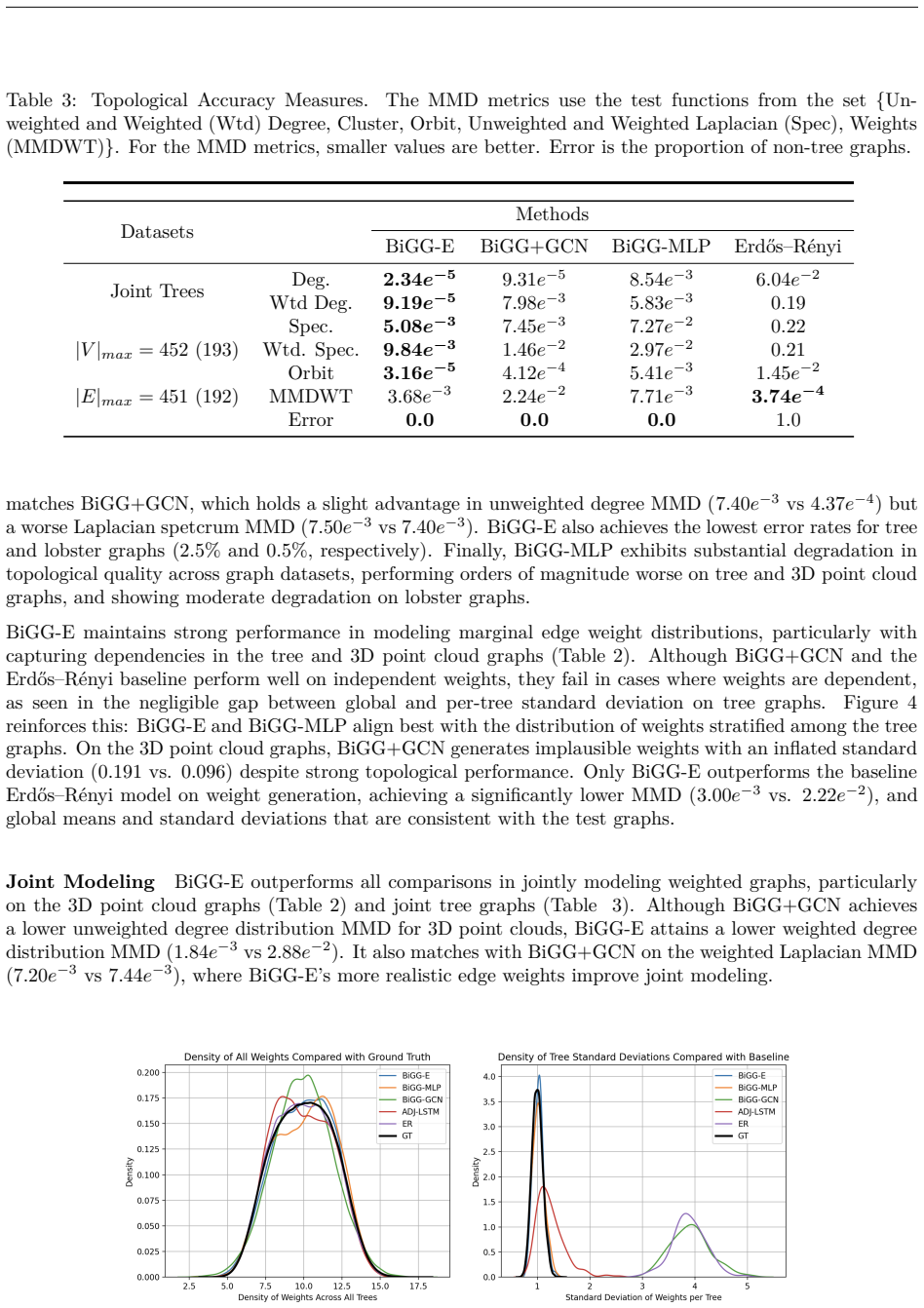
- [§4.1, Table 1 (3D Point Cloud row)] The text states that BiGG+GCN holds a "slight advantage" in unweighted degree MMD for the 3D Point Cloud dataset, but the reported values are 7.40e-3 for BiGG-E versus 4.37e-4 for BiGG+GCN: a 17-fold gap, not a slight one. This is difficult to reconcile with the abstract's claim that BiGG-E "best captures distributions over weighted graphs." The claim should be qualified to the metrics that BiGG-E actually leads, or the discrepancy should be analyzed and explained.
- [Tables 1–3 and Section 4.1] All reported MMD values, error rates, means, and standard deviations are single point estimates; no standard errors, confidence intervals, or repeated-seed results are given. This is a load-bearing issue for the empirical claim that BiGG-E "consistently outperforms" the alternatives, because several differences are small (e.g., Table 1 Tree Deg. 2.94e-6 vs 8.47e-6) and some comparisons go the other direction (e.g., Table 2 Erdős–Rényi MMDWT 6.83e-3 for BiGG-E vs 3.01e-3 for the ER baseline). Please report variability across seeds or otherwise provide a statistical basis for the comparative claims.
- [§3.4.1 and Algorithm 1] The notation w0_k = LSTMθ(wk) is ambiguous. If this is the standard recurrent LSTM, the sequence of weight embeddings has a sequential dependence over k, so computing all w0_k during training would require O(m) time, which contradicts the claimed O(log n) training time. If instead the operation is a per-weight feedforward embedding that happens to use LSTM-style gates on a single input, the paper should say so explicitly and not describe it as a recurrent LSTM. Please clarify the computation and provide the training-time complexity of the weight Fenwick-tree construction under the intended interpretation.
minor comments (5)
- [§2.1] The canonical-ordering approximation p(G) ≈ p(|V| = n)p(W_π(G)) is acknowledged but not discussed as a limitation. Since the learned distribution is not permutation invariant under arbitrary node orderings, it would be helpful to state this explicitly and comment on when the canonical ordering is meaningful for the benchmark datasets.
- [§3.1] The notation ε|e ∼ N(µ, σ) should specify the variance parameter: either N(µ, σ²) or N(µ, σ) with σ denoting standard deviation, and then Equation (3) should use the same convention consistently.
- [§4.1, Scalability paragraph] The text says "In Figure 4, we empirically demonstrate that all BiGG extensions remain efficient," but Figure 4 shows weight distributions; the scalability plots are in Figure 5. Please correct the cross-reference.
- [Algorithm 1, line 9] The return value "{edge indext represents}" appears to be a garbled placeholder. It should be replaced with a concrete symbolic representation of the sampled edge index.
- [Tables 1 and 2] There are formatting issues in the tables, including "0 .76", "0 .065", and "Erdos Renyi" in Table 2. These should be cleaned up for the final version.
Circularity Check
No significant circularity: BiGG-E's weighted-graph extension is compositional, parameter-counted, and evaluated against held-out external benchmarks.
full rationale
BiGG-E's derivation chain is not circular. The joint distribution over topology and weights is obtained by the ordinary product rule in Eq. 2, and the likelihoods in Eqs. 4, 5, 13, and 14 are chain-rule factorizations over matrix entries or over the edge set, with the weight term being the stated softplus-normal density described in Section 3.1. The asymptotic claims are count-based: the Fenwick topology tree gives O(log n) training and O((n + m) log n) sampling in BiGG (Dai et al., 2020), and the added Fenwick weight tree is analyzed separately in Sections 3.4.1 and 3.4.3 as O(log m) training and O(m log m) sampling. None of these rates is fitted to the benchmark metrics. The empirical evaluations use held-out test graphs and MMD statistics on degree, clustering, orbit, Laplacian spectrum, weighted degree, and weight marginals (Tables 1-4); these metrics are not terms in the training objective, so no fitted parameter is relabeled as a prediction. The canonical-ordering approximation p(G) = p(|V|=n) p(W_pi(G)) is explicitly presented as an intractability-motivated lower bound inherited from Liao et al. (2019) and Dai et al. (2020), not as a derived exact equivalence. The paper's only author self-citation (Baele et al., 2025, listed as an application domain) is not load-bearing. A non-circular correctness concern remains: Eq. 3 prints 1/(2 * sigma^2) where the softplus-normal density has (sqrt(2*pi)*sigma)^{-1} times the w-only Jacobian e^w/(e^w - 1); if implemented verbatim, the sigma estimate would be biased, but this is an implementation or likelihood bug, not a self-referential reduction. No circular step is present.
Assumptions & free parameters
free parameters (4)
- Softplus-normal location mu =
learned via MLP f_mu
- Softplus-normal scale sigma =
learned via MLP f_sigma2
- Weight loss scaling factor =
10, increased to 100 after plateau
- Weight state embedding dimension =
16 for quality runs, 32 for scalability runs
assumptions (4)
- domain assumption Chain rule factorization of the weighted graph distribution p(G) = p(|V|) p(W_pi(G)) under a canonical ordering.
- domain assumption Graphs are sparse, m = O(n), so sampling time is O((n+m) log n).
- ad hoc to paper The softplus-normal distribution is flexible enough to model the edge-weight distributions in the benchmarks.
- standard math Standard Fenwick tree operations run in O(log n) time.
Cite this review
Pith. "Pith review of Scalable Generative Modeling of Weighted Graphs." pith.science (2026). https://pith.science/paper/Y636KU3A
@misc{pith2026250723111,
  author       = {Pith},
  title        = {Pith review of: Scalable Generative Modeling of Weighted Graphs},
  year         = {2026},
  howpublished = {\url{https://pith.science/paper/Y636KU3A}},
  note         = {Machine review of arXiv:2507.23111}
}
abstract
Weighted graphs are ubiquitous throughout biology, chemistry, and the social sciences, motivating the development of generative models for abstract weighted graph data using deep neural networks. However, most current deep generative models are either designed for unweighted graphs and are not easily extended to weighted topologies or incorporate edge weights without consideration of a joint distribution with topology. Furthermore, learning a distribution over weighted graphs must account for complex nonlocal dependencies between both the edges of the graph and corresponding weights of each edge. We develop an autoregressive model BiGG-E, a nontrivial extension of the BiGG model, that learns a joint distribution over weighted graphs while still exploiting sparsity to generate a weighted graph with $n$ nodes and $m$ edges in $O((n + m)\log n)$ time. Simulation studies and experiments on a variety of benchmark datasets demonstrate that BiGG-E best captures distributions over weighted graphs while remaining scalable and computationally efficient.
Figures


Figures from the paper (2 more)

Forward citations
Cited by 1 Pith paper
-
TVGL-CFM:Generating and Forecasting Time-Varying Trajectories of Dynamic Networks with Conditional Flow Matching
TVGL-CFM generates and forecasts time-varying precision-matrix trajectories with flow matching in a log-Euclidean chart, outperforming raw-signal baselines on EEG, chaotic, and gene-expression data.
Reference graph
Works this paper leans on
-
[1]
First, because all decision treesTu are known a priori during training, bottom-up summaries are computed from the leaves to the root of each tree. Importantly, the summary state for each row is independent of those for other rows, allowing these computations to be performed in parallel
-
[2]
Next, using the root-level summaries from eachTu, the model computes internal nodesgi j of the Fenwick topology tree in a level-wise manner using equation 16
-
[3]
Once the Fenwick topology tree is constructed, BiGG concurrently computes the row summary states hrow u in parallel using equation 17
-
[4]
Finally, we note that for graph generation, the treesTu must be constructed sequentially
Finally, given each row-level summaryhrow u , the model computes all left and right edge existence probabilities in parallel, traversing from the root to the leaves of each tree, as defined in equation 15. Finally, we note that for graph generation, the treesTu must be constructed sequentially. However, eachTu can still be built inO(logn) time, reducing t...
work page 2018
-
[6]
hR, hC∈ Rhdim =⇒ h∈ R2hdim and Wh∈ R2hdim×2hdim
-
[7]
xij∈ Ridim =⇒ Wi∈ R2hdim×idim
-
[8]
b∈ R2hdim. Hence, we can partition the weight matrices and bias vector from the LSTM equations by defining the following partitions for each weight matrix: Wx = [UR UC ] (18) 22 Table 5: Performance on updating the states simultaneously (“Joint“) vs separately (“Independent“) Update Mode Deg. Clus. Top Spec. Wt. Spec. MMDWt Error Joint 2.46e−4 0.0 9 .98e−...
-
[9]
µk∼U (7, 13) =⇒ E(µk) = 10 and Var(µk) = 3
Show all 12 references
-
[10]
Next, an application of iterative expectation and variance yield the mean and variance of weights pooled from all trees as
wij∼ Γ(µ2 k,µ−1 k ) =⇒ E(wij|µk) =µk and Var(wij|µk) = 1 Importantly, the variance of the weights found in each tree is free of the parameterµk. Next, an application of iterative expectation and variance yield the mean and variance of weights pooled from all trees as
-
[11]
E (wij) = Eµ[Ew(wij|µk)] = Eµ(µk) = 10
-
[12]
23 A.5 Further Training Details Hyperparameters For Adj-LSTM, node states were parameterized with a hidden dimension of 128 and use a 2-layer LSTM
Var(wij) = Eµ[Varw(wij|µk)] +Varµ[Ew(wij|µk)] = Eµ(1 ) +Varµ(µk) = 1 + 3 = 4 Thus, to test for autoregressiveness in the models, we observe that weights pooled from all trees have variance Var(wij) = 4, whereas weights from a single tree have variance Var(wij|µk) = 1. 23 A.5 F...
2018
-
[1997]
John Ingraham, Vikas Garg, Regina Barzilay, and Tommi Jaakkola
doi: 10.1162/neco.1997.9.8.1735. John Ingraham, Vikas Garg, Regina Barzilay, and Tommi Jaakkola. Generative models for graph- based protein design. In H. Wallach, H. Larochelle, A. Beygelzimer, F. d 'Alché-Buc, E. Fox, and R. Garnett (eds.), Advances in Neural Information Proc...
2018 arXiv
Reviewed August 6, 2026 · model on record in the stance chip above.
Discussion (0). Continue with ORCID to comment.