REVIEW 3 major objections 6 minor 101 references
Unveiling the Atmosphere of HR 7672 B from the Near-Infrared High-Resolution Spectrum Using REACH/Subaru
T0 review · 3 major / 6 minor · reviewed 2026-08-06 · deepseek-v4-flash
Pith's one-line read High-resolution REACH spectra of the L4.5 brown dwarf HR 7672 B show water and iron hydride absorption and require an optically thick cloud deck near 14 bar.
desk verdict A credible first REACH science paper whose telluric model is the one soft spot; the detections and cloudy preference are likely robust, and it deserves a serious referee. read the letter →
The pith
A machine-rendered reading of the paper's core claim, the machinery that carries it, and where it could break.
The reading
What carries the argument
The load-bearing machinery is a single autodifferentiable spectral model that simultaneously computes the brown dwarf spectrum, telluric transmission, and host-star leakage. The brown dwarf part uses a power-law temperature–pressure profile, constant volume-mixing-ratio opacities for water and iron hydride, collision-induced absorption, and a two-parameter cloud: a fixed, optically thick opacity ($\tau_\mathrm{cloud}=500$) inserted at pressures $P>P_\mathrm{top}$. Telluric transmission is modelled as the exponential of summed cross-sections for $\mathrm{H_2O}$, $\mathrm{CO_2}$, $\mathrm{CH_4}$, and $\mathrm{O_2}$ at fixed summit pressure and temperature, with a free Doppler shift. Host-star light is treated as a scaled version of the observed HR 7672 A spectrum. The model is fit jointly to the J-band photometric magnitude and the high-resolution spectra using Hamiltonian Monte Carlo with a jitter term, and the molecular detections are cross-checked with cross-correlation functions built from the best-fit model.
What would settle it
Re-analyse the two nights of data after dividing out the telluric absorption using a rapidly rotating standard star observed on the same night; if the retrieved H2O and FeH mixing ratios or the cloud-top pressure shift by more than the quoted uncertainties, the fixed-T-P telluric model is falsified.
Extended reading notes
Core claim
The central claim is that the J- and H-band spectrum of HR 7672 B is dominated by water ($\mathrm{H_2O}$) and iron hydride ($\mathrm{FeH}$) absorption, and that a wavelength-independent continuum source—an optically thick cloud at $P_\mathrm{top} = 10^{1.16}\,\mathrm{bar}\simeq14\,\mathrm{bar}$ with a cloud-top temperature near 2112 K—is required to reproduce the observed features. A cloud-free model can also fit the data, but only by letting collision-induced absorption supply the continuum, and the cloudy model is favoured by $\Delta\mathrm{BIC}\simeq22$. The retrieved temperature–pressure profile places the cloud top between the condensation curves of $\mathrm{TiO_2}$, $\mathrm{Al_2O_3}$, and Fe, making those the likely cloud materials. Cross-correlation analysis independently confirms the molecular detections, with S/N of 3.6 for $\mathrm{FeH}$ in the J band and 6.9 for $\mathrm{H_2O}$ in the H band. The paper also presents the first characterization of the periodic noise systematics that currently limit REACH's usable wavelength range.
Load-bearing premise
The analysis assumes the model of Earth's telluric absorption—computed at fixed temperature and pressure and fitted simultaneously with the brown dwarf spectrum—is accurate enough that its deviations of up to 0.1 in normalized flux around some telluric lines do not bias the retrieved molecular abundances or cloud-top pressure.
Editorial extensions
If this is right
- REACH can deliver molecular detections and cloud-top constraints for faint companions at $R\sim100{,}000$, complementing K-band high-resolution instruments by probing deeper atmospheric layers near 4–15 bar.
- The retrieved water abundance (log VMR $\simeq -3.8$) is consistent within $3\sigma$ with the earlier K-band retrieval, supporting a uniform composition across the altitudes probed by the two bands.
- A cloud-top temperature near 2110 K provides a concrete benchmark for cloud-condensation models of L dwarfs, pointing to $\mathrm{TiO_2}$, $\mathrm{Al_2O_3}$, or Fe grains.
- Characterizing the periodic noise systematics gives future REACH users a template for mitigating fringing-like signals in post-processing, which will extend the usable spectral range toward the longer H band.
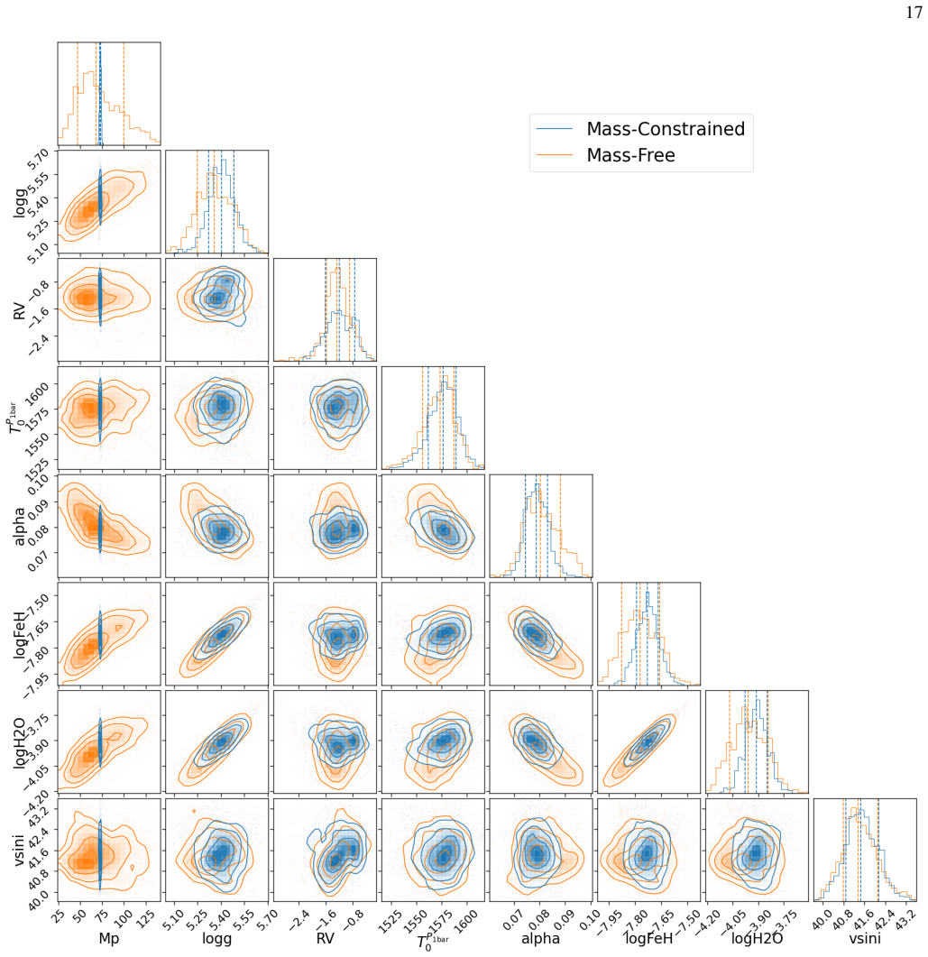
- In the mass-free cloudy retrieval, the mass upper limit is unconstrained, indicating that for cloudy atmospheres J/H-band spectra alone may not pin down surface gravity when cloud opacity hides the collision-induced continuum.
Reading between the lines
- If the retrieved cloud is as optically thick as assumed, the J-band continuum should be nearly grey; a test would be to compare the continuum slope across the full J band with the cloudy and clear-sky models fit to future full-band data.
- The paper's 3.3σ shortfall of retrieved water relative to thermochemical equilibrium could reflect vertical mixing or a non-constant abundance profile that the constant-VMR assumption cannot capture; a per-order or per-night jackknife could reveal whether residual telluric error drives the deficit.
- An empirical check of the telluric model—dividing the companion spectra by a same-night rapidly rotating standard star instead of forward-modelling telluric lines—would directly test the paper's weakest assumption; agreement would strengthen the cloud claim, disagreement would implicate telluric systematics.
- The same joint modelling of companion, host-star leakage, and telluric transmission is a natural template for future REACH observations of directly imaged exoplanets, provided the targets rotate slowly enough to resolve molecular line structure.
Editorial analysis
A structured set of objections, weighed in public.
Referee Report
Summary. This paper presents the first atmospheric retrieval from REACH/Subaru high-resolution spectra (R ~ 100,000 in Y, J, H) of the benchmark L4.5 brown dwarf HR 7672 B. The forward model is built on ExoJAX and simultaneously treats brown-dwarf molecular opacity (H2O, FeH, CIA), a simplified optically thick cloud, telluric transmission, host-star light leakage, and a low-order continuum correction. The authors run four HMC retrievals (mass-constrained/free x cloudy/clear) over narrow J- and H-band windows and report detections of H2O and FeH, a cloud-top pressure log10(Ptop/bar) ~ 1.16, a cloud-top temperature near 2112 K, and a strong preference for the cloudy model (Delta BIC ~ 22). The molecular identifications are supported by a null-test cross-correlation procedure (Appendix B), and the paper also characterizes periodic noise in REACH faint-target spectra.
Significance. If the results hold, this paper demonstrates that high-contrast, high-resolution YJH spectroscopy with REACH can recover molecular abundances and cloud properties for a faint companion at 0.7 arcsec separation, a useful step for the field. The work benefits from a benchmark target with a dynamical mass, a publicly archived retrieval code and data (Zenodo/GitHub), and an explicit null test for CCF-based molecular detection. The comparison with the KPIC/Keck retrieval of Wang et al. (2022) is appropriate and places the new abundance and T-P constraints in context. The central atmospheric conclusions, however, rest on two assumptions that need quantitative stress-testing: the fixed-temperature-pressure telluric model and the post-hoc selection of very narrow wavelength windows for the cloud-vs-clear comparison.
major comments (3)
- [Section 3.2 / 3.2.1, Eq. (2)] The telluric transmission model fixes T = 273 K and P = 0.6005 bar for all species and fits only column-scale factors beta_i. Section 3.2.1 reports residuals up to 0.1 in normalized flux around telluric lines, which is roughly 100 times the mean per-pixel uncertainties (7.8e-4 and 8.1e-4) quoted in Figure 2 and Section 2.1. Because the telluric model is multiplied into and fitted simultaneously with the companion model (Eq. 5), a coherent line-shape error cannot be absorbed by the beta_i and can directly bias the retrieved molecular abundances and pseudo-continuum, particularly in the H band where telluric and brown-dwarf H2O lines overlap at 1.48-1.54 um. The statement that these residuals have no significant impact because they are 'comparable to the spectral noise' is not quantitatively supported: the jitter term sigma = 0.06 (Table 2) inflates the noise but does not correct a coherent systematic. I request a robustness test that varies the telluric T-P profile, or uses per-species effective temperatures, or repeats the retrieval after masking or down-weighting the strongest telluric lines, and reports the resulting shifts in logH2O, logFeH, and logPtop. Note also that the telluric-model validation was performed on a June 6 standard-star observation, while the companion was observed on June 24; the residual budget on the science night is assumed by the analysis, not demonstrated.
- [Section 4.1.3 / Section 5.1] The cloud-formation claim rests on the wavelength dependence of the continuum, but the retrieval uses only two narrow windows (J orders 43-45, 1.265-1.3 um; H orders 57-60, 1.48-1.54 um) that were selected after inspecting the data. The Y band and the 1.57-1.67 um H-band region are excluded (Sections 2.1 and 3). With such limited coverage, the Delta BIC = 21.9 preference for the cloudy model may reflect the particular choice of windows rather than a real, robust continuum shape. Please demonstrate that the cloud-vs-clear conclusion is stable to the inclusion or removal of wavelength ranges, or use injected cloud models to calibrate the sensitivity of this BIC comparison under the present spectral coverage.
- [Section 3.4.2] The J-band host-star leakage is fixed at 63% based on a retrieval around the single Paschen-beta line, with the stated expectation that deviations are absorbed by the linear trend parameter a in Eq. (6). A single-line measurement, combined with the assumption that the telluric transmission is identical on the two nights (TA = TB), is a fragile anchor for a parameter that directly sets the J-band continuum level and therefore affects the retrieved FeH abundance and line-to-continuum ratios. I recommend running a sensitivity test in which log(scale_star_y) is a free parameter and reporting the resulting change in logFeH and logPtop; if the degeneracy with the linear correction is strong, the abundance uncertainties should be enlarged accordingly.
minor comments (6)
- [Table 1 / Table 2] The notation T_1bar^0 and T^Ptop_0 is easy to confuse in the tables; please define the reference pressure explicitly in the table caption for each quantity.
- [Figure 2] The pink wavelength ranges used in the retrieval are difficult to distinguish in the printed figure; consider adding shaded vertical bands spanning both panels in each wavelength window.
- [Section 4.1.1 / Appendix B] The overall CCF peak S/N = 11.4 is quoted in the main text, but the molecular S/N values of 3.6 (FeH) and 6.9 (H2O) appear only in Appendix B; the main text should state these values explicitly because they are the actual detection statistics for the two species.
- [Section 3.6, Eq. (10)] The BIC formula uses the maximum of the likelihood, but the text does not specify how this maximum is obtained from the HMC posterior; please state whether it is the maximum over posterior samples or a separate optimization.
- [Section 3.2] The telluric absorber list includes O2 in the J band and H2O, CO2, and CH4 in the H band; please state explicitly whether O2 is also included in the H-band window or whether its opacity is negligible there.
- [Section 2.2 / Appendix A] The long-period noise characterization is thorough, but the paper does not translate the measured 15-22% noise amplitude into a quantitative uncertainty on the excluded 1.57-1.67 um region or on the continuum shape; a one-sentence quantitative summary would help readers judge the impact of the wavelength selection.
Circularity Check
No load-bearing circularity; the only mild issue is that a fitted photometric point is retrospectively labeled a prediction.
-
fitted input called prediction
[Section 4.1.1 (Results from a Cloudy Model), with the fitting setup in Section 3 and Equation (7).]
"The prediction of the J-band magnitude is 14.48, with a 95 % credible interval of [13.86, 14.98]. This range includes the observed J-band magnitude of 14.39 ± 0.20."
The observed J-band magnitude is not a withheld test point: Section 3 states that 'we computed the J-band photometric magnitude and fitted it to the magnitudes observed by Boccaletti et al. (2003)', and Equation (7) includes (D_J - M_J)^2 in the likelihood. The posterior predictive value for M_J is therefore conditioned on D_J, so its interval enclosing D_J is expected by construction rather than being an independent prediction. This is a minor rhetorical overstatement; the central H2O/FeH and cloud claims are not based on this 'prediction'.
full rationale
The paper's central derivations are self-contained inversions rather than circular constructions. The retrieval fits a high-resolution spectral model to the J/H-band data and then reports the fitted H2O and FeH abundances and cloud-top pressure; these are explicitly labeled retrieval results, not independent predictions. The CCF detections in Section 4.1.1 and Appendix B use templates from the best-fit model but include a genuine null test: the cross-correlation with the residual after subtracting the full model shows no peak, while the residual against the model without the target molecule shows a peak. This makes the molecular attribution an internal consistency check rather than a definitional tautology. The cloud preference is established by a BIC model comparison (Delta BIC ~ 21.9) between a cloudy model with a free Ptop and a clear-sky model, and the paper explicitly notes that the clear-sky model can also fit the spectra, so the cloudy conclusion is not forced by the parameterization. The self-citations (ExoJAX/Kawahara et al. 2022, 2025; Kawashima et al. 2025) are tool use, prior methodological precedent, or comparison, not load-bearing uniqueness arguments. The fixed-T/P telluric model with residuals up to 0.1 is a genuine systematic-error risk for the reported abundances and cloud-top pressure, but it is a correctness limitation, not a circular step, because no telluric parameter is defined in terms of the retrieved brown dwarf properties. The only mild circularity is the retrospective labeling of the fitted J-band magnitude as a 'prediction'.
Assumptions & free parameters
free parameters (10)
- H2O volume mixing ratio (log10) =
-3.83 (+0.09/-0.07)
- FeH volume mixing ratio (log10) =
-7.41 (+0.10/-0.09)
- Temperature at cloud top (T_Ptop) =
2112 K (+46/-49)
- Power-law index alpha =
0.12 (+0.02/-0.01)
- Surface gravity log g =
5.46 (+0.09/-0.09)
- Projected rotation speed vsin(i) =
41.28 km/s (+0.92/-0.61)
- Cloud top pressure log10(Ptop/bar) =
1.16 (+0.08/-0.08)
- Host star leakage in H band (log scale_star_h) =
-0.43 (+0.02/-0.02)
- Telluric column coefficients (log beta H2O, CO2, CH4, O2) =
21.48, 21.28, 17.49, 24.20
- Jitter term sigma =
0.06
assumptions (7)
- domain assumption Volume mixing ratios are constant with pressure for H2O and FeH.
- domain assumption The T-P profile follows a power law T(P)=T0(P/P0)^alpha with 300 layers.
- domain assumption Cloud opacity is modeled as an optically thick layer with tau_cloud=500 fixed.
- domain assumption Telluric transmission is modeled with fixed pressure and temperature (0.6005 bar, 273 K).
- domain assumption Host star contamination can be represented by scaling the observed HR 7672 A spectrum with a single factor, and telluric transmission is identical for A and B observations.
- domain assumption Line lists (POKAZATEL, MoLLIST, etc.) and CIA coefficients from HITRAN are accurate in the modeled bands.
- standard math The HMC-NUTS sampling with 1000 post-warmup samples and R-hat below 1.1 indicates convergence.
Cite this review
Pith. "Pith review of Unveiling the Atmosphere of HR 7672 B from the Near-Infrared High-Resolution Spectrum Using REACH/Subaru." pith.science (2026). https://pith.science/paper/RMMXRHPS
@misc{pith2026250801281,
  author       = {Pith},
  title        = {Pith review of: Unveiling the Atmosphere of HR 7672 B from the Near-Infrared High-Resolution Spectrum Using REACH/Subaru},
  year         = {2026},
  howpublished = {\url{https://pith.science/paper/RMMXRHPS}},
  note         = {Machine review of arXiv:2508.01281}
}
abstract
Characterizing the atmospheres of exoplanets and brown dwarfs is crucial for understanding their atmospheric physics and chemistry, searching for biosignatures, and investigating their formation histories. Recent advances in observational techniques, combining adaptive optics with high-resolution spectrographs, have enabled detailed spectroscopic analysis for directly imaged faint companions. In this paper, we report an atmospheric retrieval on the L-type brown dwarf HR 7672 B using a near-infrared high-contrast high-resolution spectrograph, REACH (Y, J, H band, $R\sim100,000$), which combines SCExAO with IRD at the Subaru Telescope. Our model, developed based on the ExoJAX spectrum code, simultaneously accounts for several factors, including the presence of clouds in the L dwarf's atmosphere as well as contamination from the host star's light and telluric absorption lines in the observed spectra. Our analysis identified H2O and FeH as the primary absorbers in the observed J- and H-band spectra. Additionally, the observed features were reproduced with a model that includes cloud opacity, assuming an optically thick cloud at the pressure $P_\mathrm{top}$. The resulting temperature at the cloud top pressure suggests the potential formation of clouds composed of TiO2, Al2O3, or Fe. This study is the first science demonstration for faint spectra obtained by REACH, providing a foundation for future investigations into the atmospheres of exoplanets and brown dwarfs.
Figures


Figures from the paper (15 more)




Reference graph
Works this paper leans on
-
[1]
2014, in Society of Photo-Optical Instrumentation Engineers (SPIE) Conference Series, V ol
Artigau, ´E., Astudillo-Defru, N., Delfosse, X., et al. 2014, in Society of Photo-Optical Instrumentation Engineers (SPIE) Conference Series, V ol. 9149, Observatory Operations:
2014
-
[2]
Strategies, Processes, and Systems V , ed. A. B. Peck, C. R. Benn, & R. L. Seaman, 914905, doi: 10.1117/12.2056385 Astropy Collaboration, Robitaille, T. P., Tollerud, E. J., et al. 2013, A&A, 558, A33, doi: 10.1051/0004-6361/201322068 28 Astropy Collaboration, Price-Whelan, A. M., Sip˝ocz, B. M., et al. 2018, AJ, 156, 123, doi: 10.3847/1538-3881/aabc4f As...
-
[3]
2018, VizieR Online Data Catalog, I/347
Andrae, R. 2018, VizieR Online Data Catalog, I/347
2018
-
[4]
Baraffe, I., Chabrier, G., Allard, F., & Hauschildt, P. H. 1998, A&A, 337, 403, doi: 10.48550/arXiv.astro-ph/9805009
-
[5]
Barman, T. S., Konopacky, Q. M., Macintosh, B., & Marois, C. 2015, ApJ, 804, 61, doi: 10.1088/0004-637X/804/1/61
-
[6]
S., Macintosh, B., Konopacky, Q
Barman, T. S., Macintosh, B., Konopacky, Q. M., & Marois, C. 2011, ApJ, 733, 65, doi: 10.1088/0004-637X/733/1/65
-
[7]
2019, AJ, 158, 164, doi: 10.3847/1538-3881/ab40a7
Luger, R. 2019, AJ, 158, 164, doi: 10.3847/1538-3881/ab40a7
-
[8]
Bernath, P. F. 2020, J. Quant. Spec. Radiat. Transf., 240, 106687, doi: 10.1016/j.jqsrt.2019.106687
arXiv 2020
Show all 101 references
-
[9]
L., Lallement, R., Ferron, S., Boonne, C., & Bodichon, R
Bertaux, J. L., Lallement, R., Ferron, S., Boonne, C., & Bodichon, R. 2014, A&A, 564, A46, doi: 10.1051/0004-6361/201322383
2014 doi
- [10]
-
[11]
M., & Marchis, F
Boccaletti, A., Chauvin, G., Lagrange, A. M., & Marchis, F. 2003, A&A, 410, 283, doi: 10.1051/0004-6361:20031216
2003 doi
-
[12]
P., Tran, Q
Bowler, B. P., Tran, Q. H., Zhang, Z., et al. 2023, AJ, 165, 164, doi: 10.3847/1538-3881/acbd34
2023 doi
-
[13]
2018, JAX: composable transformations of Python+NumPy programs, 0.3.13
Bradbury, J., Frostig, R., Hawkins, P., et al. 2018, JAX: composable transformations of Python+NumPy programs, 0.3.13. http://github.com/google/jax
2018
-
[14]
D., Dupuy, T
Brandt, T. D., Dupuy, T. J., & Bowler, B. P. 2019, AJ, 158, 140, doi: 10.3847/1538-3881/ab04a8
2019 doi
-
[15]
M., Fischer, D
Brewer, J. M., Fischer, D. A., Valenti, J. A., & Piskunov, N. 2016, ApJS, 225, 32, doi: 10.3847/0067-0049/225/2/32
2016 doi
-
[16]
2017, Geomorphology, 282, 131, doi: 10.1016/j.geomorph.2016.12.029
Burningham, H., & French, J. 2017, Geomorphology, 282, 131, doi: 10.1016/j.geomorph.2016.12.029
2017 doi
-
[17]
Burrows, A. S. 2014, Proceedings of the National Academy of Science, 111, 12601, doi: 10.1073/pnas.1304208111
2014 doi
-
[18]
2007, A&A, 467, 777, doi: 10.1051/0004-6361:20066514
Casali, M., Adamson, A., Alves de Oliveira, C., et al. 2007, A&A, 467, 777, doi: 10.1051/0004-6361:20066514
2007 doi
-
[19]
2000, ApJ, 542, 464, doi: 10.1086/309513
Chabrier, G., Baraffe, I., Allard, F., & Hauschildt, P. 2000, ApJ, 542, 464, doi: 10.1086/309513
2000 doi
-
[20]
2023, A&A, 671, A119, doi: 10.1051/0004-6361/202243832
Chabrier, G., Baraffe, I., Phillips, M., & Debras, F. 2023, A&A, 671, A119, doi: 10.1051/0004-6361/202243832
2023 doi
-
[21]
W., & Hunten, D
Chamberlain, J. W., & Hunten, D. M. 1987, Theory of planetary atmospheres. An introduction to their physics andchemistry., V ol. 36
1987
-
[22]
A., Shephard, M
Clough, S. A., Shephard, M. W., Mlawer, E. J., et al. 2005, J. Quant. Spec. Radiat. Transf., 91, 233, doi: 10.1016/j.jqsrt.2004.05.058
2005 doi
-
[23]
R., Johnson, J
Crepp, J. R., Johnson, J. A., Fischer, D. A., et al. 2012, ApJ, 751, 97, doi: 10.1088/0004-637X/751/2/97
2012 doi
-
[24]
C., Rayner, J
Cushing, M. C., Rayner, J. T., & Vacca, W. D. 2005, ApJ, 623, 1115, doi: 10.1086/428040
2005 doi
-
[25]
2020, in Society of Photo-Optical Instrumentation Engineers (SPIE) Conference
Delorme, J.-R., Jovanovic, N., Echeverri, D., et al. 2020, in Society of Photo-Optical Instrumentation Engineers (SPIE) Conference
2020
-
[26]
11447, Ground-based and Airborne Instrumentation for Astronomy VIII, ed
Series, V ol. 11447, Ground-based and Airborne Instrumentation for Astronomy VIII, ed. C. J. Evans, J. J. Bryant, & K. Motohara, 114471P, doi: 10.1117/12.2562836
-
[27]
2021, Journal of Astronomical Telescopes, Instruments, and Systems, 7, 035006, doi: 10.1117/1.JATIS.7.3.035006
Delorme, J.-R., Jovanovic, N., Echeverri, D., et al. 2021, Journal of Astronomical Telescopes, Instruments, and Systems, 7, 035006, doi: 10.1117/1.JATIS.7.3.035006
2021 doi
-
[28]
T., Friberg, P., Jenness, T., et al
Dempsey, J. T., Friberg, P., Jenness, T., et al. 2013, MNRAS, 430, 2534, doi: 10.1093/mnras/stt090
2013 doi
-
[29]
W., Burrows, A., et al
Dulick, M., Bauschlicher, Jr., C. W., Burrows, A., et al. 2003, ApJ, 594, 651, doi: 10.1086/376791
2003 doi
-
[30]
1996, ApJ, 472, L37, doi: 10.1086/310356
Fegley, Bruce, J., & Lodders, K. 1996, ApJ, 472, L37, doi: 10.1086/310356
1996 doi
-
[31]
2016, The Journal of Open Source Software, 1, 24, doi: 10.21105/joss.00024
Foreman-Mackey, D. 2016, The Journal of Open Source Software, 1, 24, doi: 10.21105/joss.00024
2016 doi
- [32]
-
[33]
B., Stern, H
Gelman, A., Carlin, J. B., Stern, H. S., et al. 2014, Bayesian Data Analysis
2014
-
[34]
R., Line, M
Gharib-Nezhad, E., Iyer, A. R., Line, M. R., et al. 2021, ApJS, 254, 34, doi: 10.3847/1538-4365/abf504
2021 doi
-
[35]
M., Brasseur, C
Ginsburg, A., Sip˝ocz, B. M., Brasseur, C. E., et al. 2019, AJ, 157, 98, doi: 10.3847/1538-3881/aafc33
2019 doi
-
[36]
E., Rothman, L
Gordon, I. E., Rothman, L. S., Hargreaves, R. J., et al. 2022, J. Quant. Spec. Radiat. Transf., 277, 107949, doi: 10.1016/j.jqsrt.2021.107949
2022
-
[37]
Z., Pueyo, L., Ruffio, J.-B., et al
Greenbaum, A. Z., Pueyo, L., Ruffio, J.-B., et al. 2018, AJ, 155, 226, doi: 10.3847/1538-3881/aabcb8
2018 doi
-
[38]
A., Yelle, R
Griffith, C. A., Yelle, R. V ., & Marley, M. S. 1998, Science, 282, 2063, doi: 10.1126/science.282.5396.2063
1998
-
[39]
2014, AJ, 148, 53, doi: 10.1088/0004-6256/148/3/53
Gullikson, K., Dodson-Robinson, S., & Kraus, A. 2014, AJ, 148, 53, doi: 10.1088/0004-6256/148/3/53
2014 doi
-
[40]
J., Gordon, I
Hargreaves, R. J., Gordon, I. E., Rey, M., et al. 2020, ApJS, 247, 55, doi: 10.3847/1538-4365/ab7a1a
2020 doi
-
[41]
J., Hinkle, K
Hargreaves, R. J., Hinkle, K. H., Bauschlicher, Jr., C. W., et al. 2010, AJ, 140, 919, doi: 10.1088/0004-6256/140/4/919
2010 doi
-
[42]
R., Millman, K
Harris, C. R., Millman, K. J., van der Walt, S. J., et al. 2020, Nature, 585, 357, doi: 10.1038/s41586-020-2649-2
2020 doi
-
[43]
2001, A&A, 376, 194, doi: 10.1051/0004-6361:20010937
Sedlmayr, E. 2001, A&A, 376, 194, doi: 10.1051/0004-6361:20010937
2001 doi
- [44]
-
[45]
A., Ruffio, J.-B., Wang, J
Horstman, K. A., Ruffio, J.-B., Wang, J. J., et al. 2024, in Ground-based and Airborne Instrumentation for Astronomy X, V ol. 13096, SPIE, 731–743
2024
-
[46]
1999, Michigan Spectral Survey, 5, 0 29
Houk, N., & Swift, C. 1999, Michigan Spectral Survey, 5, 0 29
1999
-
[47]
J., Xuan, J
Hsu, C.-C., Wang, J. J., Xuan, J. W., et al. 2024, ApJ, 971, 9, doi: 10.3847/1538-4357/ad58d3
2024 doi
-
[48]
Hunter, J. D. 2007, Computing in Science and Engineering, 9, 90, doi: 10.1109/MCSE.2007.55
2007 doi
-
[49]
2015, PASP, 127, 890, doi: 10.1086/682989
Jovanovic, N., Martinache, F., Guyon, O., et al. 2015, PASP, 127, 890, doi: 10.1086/682989
2015 doi
-
[50]
R., Bond, C
Jovanovic, N., Delorme, J. R., Bond, C. Z., et al. 2019, arXiv e-prints, arXiv:1909.04541, doi: 10.48550/arXiv.1909.04541
2019 doi
-
[51]
E., van der Avoird, A., et al
Karman, T., Gordon, I. E., van der Avoird, A., et al. 2019, Icarus, 328, 160, doi: 10.1016/j.icarus.2019.02.034
2019 doi
-
[52]
2025, Atmospheric retrieval of HR 7672 B: Python code and input data, 1.0.0, Zenodo, doi: 10.5281/zenodo.15702022
Kasagi, Y . 2025, Atmospheric retrieval of HR 7672 B: Python code and input data, 1.0.0, Zenodo, doi: 10.5281/zenodo.15702022
2025 doi
-
[53]
E., & Raftery, A
Kass, R. E., & Raftery, A. E. 1995, Journal of the American Statistical Association, 90, 773, doi: 10.1080/01621459.1995.10476572
1995
-
[54]
2015, A&A, 576, A78, doi: 10.1051/0004-6361/201423909
Kausch, W., Noll, S., Smette, A., et al. 2015, A&A, 576, A78, doi: 10.1051/0004-6361/201423909
2015 doi
-
[55]
2022, ApJS, 258, 31, doi: 10.3847/1538-4365/ac3b4d
Kawahara, H., Kawashima, Y ., Masuda, K., et al. 2022, ApJS, 258, 31, doi: 10.3847/1538-4365/ac3b4d
2022 doi
-
[56]
2025, ApJ, 985, 263, doi: 10.3847/1538-4357/adcba2
Kawahara, H., Kawashima, Y ., Tada, S., et al. 2025, ApJ, 985, 263, doi: 10.3847/1538-4357/adcba2
2025 doi
-
[57]
2025, ApJ, 988, 53, doi: 10.3847/1538-4357/adddbd
Kawashima, Y ., Kawahara, H., Kasagi, Y ., et al. 2025, ApJ, 988, 53, doi: 10.3847/1538-4357/adddbd
2025 doi
-
[58]
M., Barman, T
Konopacky, Q. M., Barman, T. S., Macintosh, B. A., & Marois, C. 2013, Science, 339, 1398, doi: 10.1126/science.1232003
2013 doi
-
[59]
2018, in Society of Photo-Optical Instrumentation Engineers (SPIE) Conference
Kotani, T., Tamura, M., Nishikawa, J., et al. 2018, in Society of Photo-Optical Instrumentation Engineers (SPIE) Conference
2018
-
[60]
10702, Ground-based and Airborne Instrumentation for Astronomy VII, ed
Series, V ol. 10702, Ground-based and Airborne Instrumentation for Astronomy VII, ed. C. J. Evans, L. Simard, & H. Takami, 1070211, doi: 10.1117/12.2311836
-
[61]
2020, in Society of Photo-Optical Instrumentation Engineers (SPIE) Conference
Kotani, T., Kawahara, H., Ishizuka, M., et al. 2020, in Society of Photo-Optical Instrumentation Engineers (SPIE) Conference
2020
-
[62]
11448, Adaptive Optics Systems VII, ed
Series, V ol. 11448, Adaptive Optics Systems VII, ed. L. Schreiber, D. Schmidt, & E. Vernet, 1144878, doi: 10.1117/12.2561755
-
[63]
C., Fischer, D
Liu, M. C., Fischer, D. A., Graham, J. R., et al. 2002, ApJ, 571, 519, doi: 10.1086/339845
2002 doi
-
[64]
2003, ApJ, 591, 1220, doi: 10.1086/375492
Lodders, K. 2003, ApJ, 591, 1220, doi: 10.1086/375492
2003 doi
-
[65]
2002, Icarus, 155, 393, doi: 10.1006/icar.2001.6740
Lodders, K., & Fegley, B. 2002, Icarus, 155, 393, doi: 10.1006/icar.2001.6740
2002
-
[66]
2006, in Astrophysics Update 2, ed
Lodders, K., & Fegley, B., J. 2006, in Astrophysics Update 2, ed. J. W. Mason, 1, doi: 10.1007/3-540-30313-8 1
2006 doi
-
[67]
Lomb, N. R. 1976, Ap&SS, 39, 447, doi: 10.1007/BF00648343
1976 doi
-
[68]
R., Barman, T., et al
Macintosh, B., Graham, J. R., Barman, T., et al. 2015, Science, 350, 64, doi: 10.1126/science.aac5891
2015 doi
-
[69]
2019, ARA&A, 57, 617, doi: 10.1146/annurev-astro-081817-051846
Madhusudhan, N. 2019, ARA&A, 57, 617, doi: 10.1146/annurev-astro-081817-051846
2019 doi
-
[70]
S., & Robinson, T
Marley, M. S., & Robinson, T. D. 2015, ARA&A, 53, 279, doi: 10.1146/annurev-astro-082214-122522
2015 doi
-
[71]
2008, Science, 322, 1348, doi: 10.1126/science.1166585
Marois, C., Macintosh, B., Barman, T., et al. 2008, Science, 322, 1348, doi: 10.1126/science.1166585
2008 doi
-
[72]
Z., Delorme, J
Mawet, D., Bond, C. Z., Delorme, J. R., et al. 2018, in Society of Photo-Optical Instrumentation Engineers (SPIE) Conference
2018
- [73]
-
[74]
S., McGovern, M
McLean, I. S., McGovern, M. R., Burgasser, A. J., et al. 2003, ApJ, 596, 561, doi: 10.1086/377636
2003 doi
-
[75]
P., van Boekel, R., et al
Molli`ere, P., Wardenier, J. P., van Boekel, R., et al. 2019, A&A, 627, A67, doi: 10.1051/0004-6361/201935470
2019 doi
-
[76]
V ., Mukherjee, S., Marley, M
Morley, C. V ., Mukherjee, S., Marley, M. S., et al. 2024, ApJ, 975, 59, doi: 10.3847/1538-4357/ad71d5
2024 doi
-
[77]
Otten, G. P. P. L., Vigan, A., Muslimov, E., et al. 2021, A&A, 646, A150, doi: 10.1051/0004-6361/202038517
2021 doi
-
[78]
Park, J. H. 1981, Atlas of absorption lines from 0 to 17 900 cm-1
1981
- [79]
-
[80]
L., Kyuberis, A
Polyansky, O. L., Kyuberis, A. A., Zobov, N. F., et al. 2018, MNRAS, 480, 2597, doi: 10.1093/mnras/sty1877
2018 doi
-
[81]
T., Cushing, M
Rayner, J. T., Cushing, M. C., & Vacca, W. D. 2009, ApJS, 185, 289, doi: 10.1088/0067-0049/185/2/289
2009 doi
-
[82]
2018, PASP, 130, 074502, doi: 10.1088/1538-3873/aac1b4
Sameshima, H., Matsunaga, N., Kobayashi, N., et al. 2018, PASP, 130, 074502, doi: 10.1088/1538-3873/aac1b4
2018 doi
-
[83]
Scargle, J. D. 1982, ApJ, 263, 835, doi: 10.1086/160554
1982 doi
-
[84]
2015, A&A, 576, A77, doi: 10.1051/0004-6361/201423932
Smette, A., Sana, H., Noll, S., et al. 2015, A&A, 576, A77, doi: 10.1051/0004-6361/201423932
2015 doi
-
[85]
W., Kitzmann, D., Patzer, A
Stock, J. W., Kitzmann, D., Patzer, A. B. C., & Sedlmayr, E. 2018, MNRAS, 479, 865, doi: 10.1093/mnras/sty1531
2018 doi
-
[86]
2012, in Society of Photo-Optical Instrumentation Engineers (SPIE) Conference
Tamura, M., Suto, H., Nishikawa, J., et al. 2012, in Society of Photo-Optical Instrumentation Engineers (SPIE) Conference
2012
-
[87]
8446, Ground-based and Airborne Instrumentation for Astronomy IV , ed
Series, V ol. 8446, Ground-based and Airborne Instrumentation for Astronomy IV , ed. I. S. McLean, S. K. Ramsay, & H. Takami, 84461T, doi: 10.1117/12.925885
-
[88]
E., Metchev, S., Hood, C
Tannock, M. E., Metchev, S., Hood, C. E., et al. 2022, MNRAS, 514, 3160, doi: 10.1093/mnras/stac1412
2022 doi
-
[89]
N., Al-Refaie, A
Tennyson, J., Yurchenko, S. N., Al-Refaie, A. F., et al. 2016, Journal of Molecular Spectroscopy, 327, 73, doi: 10.1016/j.jms.2016.05.002 The pandas development Team. 2024, pandas-dev/pandas: Pandas, v2.2.3, Zenodo, doi: 10.5281/zenodo.3509134
2016 doi
-
[90]
J., Santos, N
Ulmer-Moll, S., Figueira, P., Neal, J. J., Santos, N. C., & Bonnefoy, M. 2019, A&A, 621, A79, doi: 10.1051/0004-6361/201833282 van Kooten, M. A. M., & Izett, J. G. 2022, PASP, 134, 095001, doi: 10.1088/1538-3873/ac81ec
2019 doi
-
[91]
E., et al
Virtanen, P., Gommers, R., Oliphant, T. E., et al. 2020, Nature Methods, 17, 261, doi: 10.1038/s41592-019-0686-2
2020 doi
-
[92]
2010, ApJ, 716, 1060, doi: 10.1088/0004-637X/716/2/1060 30
Visscher, C., Lodders, K., & Fegley, Bruce, J. 2010, ApJ, 716, 1060, doi: 10.1088/0004-637X/716/2/1060 30
2010 doi
-
[93]
R., Visscher, C., Lewis, N
Wakeford, H. R., Visscher, C., Lewis, N. K., et al. 2017, MNRAS, 464, 4247, doi: 10.1093/mnras/stw2639
2017 doi
-
[94]
R., Ruffio, J.-B., et al
Wang, J., Kolecki, J. R., Ruffio, J.-B., et al. 2022, AJ, 163, 189, doi: 10.3847/1538-3881/ac56e2
2022 doi
-
[95]
J., Ruffio, J.-B., et al
Wang, J., Wang, J. J., Ruffio, J.-B., et al. 2023, AJ, 165, 4, doi: 10.3847/1538-3881/ac9f19
2023 doi
-
[96]
J., Ruffio, J.-B., Morris, E., et al
Wang, J. J., Ruffio, J.-B., Morris, E., et al. 2021, AJ, 162, 148, doi: 10.3847/1538-3881/ac1349
2021 doi
-
[97]
2021, The Journal of Open Source Software, 6, 3021, doi: 10.21105/joss.03021
Waskom, M. 2021, The Journal of Open Source Software, 6, 3021, doi: 10.21105/joss.03021
2021 doi
-
[98]
C., Hills, R
Wiedner, M. C., Hills, R. E., Carlstrom, J. E., & Lay, O. P. 2001, ApJ, 553, 1036, doi: 10.1086/320943
2001 doi
-
[99]
W., Wang, J., Ruffio, J.-B., et al
Xuan, J. W., Wang, J., Ruffio, J.-B., et al. 2022, ApJ, 937, 54, doi: 10.3847/1538-4357/ac8673
2022 doi
-
[100]
N., Mellor, T
Yurchenko, S. N., Mellor, T. M., Freedman, R. S., & Tennyson, J. 2020, MNRAS, 496, 5282, doi: 10.1093/mnras/staa1874
2020 doi
-
[101]
Zhang, Y ., Snellen, I. A. G., & Molli`ere, P. 2021, A&A, 656, A76, doi: 10.1051/0004-6361/202141502
2021 doi
Reviewed August 6, 2026 · model on record in the stance chip above.
Discussion (0). Sign in to comment.