REVIEW 3 major objections 5 minor 5 cited by
Improved limits on the 21cm signal at z=6.5-7.0 with the MWA using Gaussian information
T0 review · 3 major / 5 minor · reviewed 2026-08-06 · deepseek-v4-flash
Pith's one-line read Fitting a single Gaussian to the distribution of MWA visibilities separates the 21cm signal from non-Gaussian foreground tails, tightening the z=6.5 power-spectrum limit from (30.2 mK)^2 to (23.0 mK)^2.
desk verdict The new 21 cm limits are real but Eq. (6) combines real/imaginary variances in quadrature instead of in sum, biasing all fitted powers low by ~29% and likely reversing the claimed z=6.8 improvement. read the letter →
The pith
A machine-rendered reading of the paper's core claim, the machinery that carries it, and where it could break.
The reading
What carries the argument
The load-bearing object is the empirical distribution of visibility realisations at fixed spatial scale: each cell of the $(u,v,\eta)$ cube supplies one sample, and a Kernel Density Estimator (a kernel-smoothed histogram) models the distribution. Fitting the widest single Gaussian and equating its variance with power $P_S(k_\perp,k_\parallel)$ is the whole trick; the Gaussian amplitude is used only for the noise term. Supporting it are the 'totals minus differences' split, which removes noise-power bias, and the CDF-integrated variance over the full histogram, which serves as the blind benchmark that reproduces the older, larger limits. WODEN simulations of diffuse plus compact foregrounds s
What would settle it
Run the same pipeline on a second deep field and on a 21cm simulation with a visibly skewed brightness-temperature distribution (non-zero skew at the neutral fractions of the Greig et al. 2022 box, per Cook et al. 2024) and check whether the fitted-Gaussian variance under-recovers the true power in the EoR window by more than the quoted thermal-plus-sample-variance error. If it does\,---\,or if EoR0 and EoR1 fields analysed identically disagree\,---\,the improved limits are biased low, not merely conservative.
Extended reading notes
Core claim
A single-Gaussian fit to the histogram of gridded visibility samples isolates the Gaussian component\,---\,21cm signal, thermal noise, Gaussian foreground residue\,---\,and discards the non-Gaussian tail that inflates standard power-spectrum estimators. The fitted variance is equated with the power $P_S(k_\perp,k_\parallel)$, with noise bias removed by subtracting 'differences' from 'totals' splits. On 268 hours of MWA data this yields 2-$\sigma$ limits of $(23.0\,\mathrm{mK})^2$ EW and $(21.7\,\mathrm{mK})^2$ NS at $z=6.5$, improving on Nunhokee et al. (2025) by factors of 1.5\,--\,2, with similar gains at $z=6.8,7.0$. CDF integration over the full histogram reproduces the older limits, con
Load-bearing premise
The improvement stands or falls on the claim that the fitted Gaussian's variance equals the true 21cm power: the signal must be fully Gaussian at $z=6.5$\,--\,$7.0$, and every other component may only broaden the distribution, never narrow it or hide power in the tails the fit discards. The paper flags this as an intuition, notes that no unique Gaussian/non-Gaussian decomposition exists, and validates it with one 21cm simulation at $z=6.5$ only.
Editorial extensions
If this is right
- The same 268 hours of data now yield a best limit of $(21.7\,\mathrm{mK})^2 = 470\,\mathrm{mK}^2$ at $z=6.5$ (NS), and the EW/NS polarisation gap shrinks because the Gaussian fit preferentially removes the Galactic-plane emission that had hurt NS.
- At $z=6.8$ and $z=7.0$ the best upper limits improve by factors of roughly 1.9 and 2.0 over the prior analysis of the same dataset.
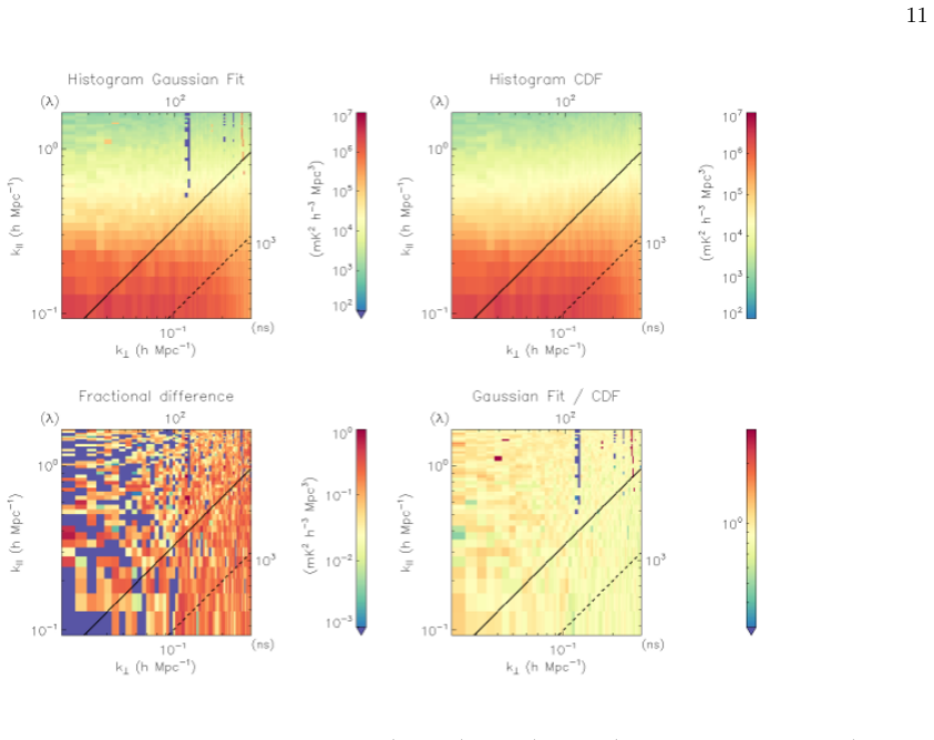
- Foreground leakage, not the 21cm signal, is identified as the source of non-Gaussianity: noise-free simulations of diffuse plus compact emission reproduce the non-Gaussian tails and the mode-dependent ratio between fitted and integrated power.
- If any additional Gaussian or non-Gaussian component only broadens the distribution, the Gaussian-fit estimate is conservative by construction\,---\,it can over-shoot the 21cm power but not, under the assumption, under-shoot it.
- The approach transfers to other foreground-dominated datasets and remains usable until the signal-to-noise regime where higher-order statistics become detectable.
Reading between the lines
- Editorial note: the abstract quotes best limits of $(25.9\,\mathrm{mK})^2$ at $z=6.8$ and $(32.0\,\mathrm{mK})^2$ at $z=7.0$, while Table 1 lists $(28.4)^2$\,--\,$(32.4)^2$ and $(35.3)^2$\,--\,$(35.4)^2$; the paper does not explain which averaging produces the abstract values.
- The $z=6.8$ and $z=7.0$ limits inherit the Gaussian-capture assumption without dedicated validation, since the 21cm simulation check is performed only at $z=6.5$; a simulation at the higher redshifts would be the cheapest test of those factors-of-two gains.
- Because the estimator needs only histograms of gridded visibilities, it could be applied to other instruments (HERA, LOFAR, SKA-Low) and to cross-checks between MWA fields without any new calibration machinery.
- The method carries a testable signature: the gap between fitted-Gaussian and CDF power should grow toward the horizon wedge and with Galactic-plane elevation, and should vanish for a 21cm-only sky.
- A second deep field analysed identically would test the anti-correlation caveat that the paper addresses only by appeal to the similar behaviour of EoR0 and EoR1.
Editorial analysis
A structured set of objections, weighed in public.
Referee Report
Summary. The manuscript proposes to estimate the Epoch of Reionization 21 cm power spectrum from MWA observations by fitting a single Gaussian to histograms of gridded visibility realisations and interpreting the fitted variance as the signal power. Non-Gaussian tails are attributed to foreground contamination and are excluded by the fit. Applying this method to 268 hours of EoR0 data, the authors report improved 2σ upper limits at z = 6.5, 6.8, and 7.0 relative to Nunhokee et al. (2025), with the largest gains at z = 6.5 for both polarizations. The method is tested against WODEN simulations of 21 cm signal alone and of signal plus foregrounds, and compared with a CDF-based estimator that uses the full histogram variance.
Significance. If the estimator is unbiased and correctly normalised, the paper offers a computationally simple way to mitigate non-Gaussian foreground leakage and could improve current MWA 21 cm limits. The inclusion of realistic foreground simulations, a 21 cm-only recovery test, and a comparison against a blind CDF estimator are clear strengths; the 21 cm-only simulation shows good agreement between the Gaussian fit and the CDF, and the foreground simulations support the interpretation that non-Gaussianity originates from foregrounds. However, the statistical combination in Eq. (6) appears to contain a normalisation error, the fitting protocol is not fully specified, and the validation is limited to a single redshift and simulation model. These issues affect the credibility of the quoted improvements and must be addressed before the limits can be accepted.
major comments (3)
- [Section 2, Eq. (6)] Equations (5) and (7) define P_S as the variance of a single real/imaginary component of the gridded visibilities. For a circular complex visibility with equal real and imaginary signal variance, the unbiased total-power estimator is [(P_tot,r + P_tot,i) - (P_diff,r + P_diff,i)]/4. Equation (6) instead combines the real and imaginary parts in quadrature: sqrt(P_tot,r^2+P_tot,i^2) - sqrt(P_diff,r^2+P_diff,i^2). For equal real/imag entries this yields a factor sqrt(2)/2 ≈ 0.707 in power, i.e. a ~29% low bias. The z=6.8 EW limit improves on Nunhokee et al. (2025) by only 21% in power, so this correction would reverse that particular comparison. The 21 cm simulation validation in Figs. 10-12 cannot detect this bias if both the fitted-Gaussian and CDF pipelines use the same Eq. (6). Please confirm whether the printed formula matches the actual analysis and, if not, recompute all quoted limits
- [Section 1 and Section 2, Gaussian fitting procedure] The paper states in the Introduction that the authors 'fit the widest Gaussian that is consistent with a Gaussian fit to the bulk of the distribution,' but Section 2 says the parameters are fitted using the IDL GAUSSFIT routine. These two descriptions are not equivalent: a standard least-squares fit to the full histogram is not the same as selecting the widest Gaussian consistent with a central bulk. The estimator's output depends on this choice, yet no operational definition or sensitivity analysis is provided for how 'widest' is determined or how tail clipping/outlier rejection is applied. The reported robustness tests cover the histogram abscissa range, bin resolution, and KDE width h, but not the fitting target. Please specify the algorithm precisely and demonstrate that the quoted limits are stable under reasonable choices.
- [Section 5 and Section 6, redshift extrapolation] The unbiasedness of the Gaussian-fit variance is validated only at z=6.5 using a single 21 cm simulation (Greig et al. 2022), while the z=6.8 and z=7.0 limits in Table 1 rest on the same assumption without dedicated validation. The paper's own Section 5 notes that the z=6.5 simulation has a 40-45% neutral fraction and Cook et al. (2024) find non-zero skew at these redshifts; the argument in Section 6 that any non-Gaussian signal would broaden the distribution is a reasonable prior but not a quantitative test. Given that the z=6.8 EW improvement is marginal even before the Eq. (6) correction, the absence of a simulation test at z=6.8/7.0 (or an explicit systematic error term) is a substantive gap. Please either extend the validation to the higher redshifts or add a conservative systematic floor to those limits.
minor comments (5)
- [Figure 7 caption] The caption describes the Nunhokee et al. (2025) result as using 'a subset of 6,395 observations,' while the text and Table 1 refer to that work as using the full 8,036-observation dataset. Please clarify which dataset the comparison limit is drawn from.
- [Abstract and Table 1] The abstract reports best limits of (25.9 mK)^2 at z=6.8 and (32.0 mK)^2 at z=7.0, but Table 1 does not contain these values: the best z=6.8 entries are (28.4 mK)^2 (EW) and (32.4 mK)^2 (NS), and the best z=7.0 entries are (35.4 mK)^2 and (35.3 mK)^2. The abstract values should be reconciled with the table.
- [Section 2, Eq. (5)] Equation (5) equates an analytic Gaussian to the KDE-weighted sum of kernels. This is a fitting relation, not an identity; please clarify the normalisation of the weights w_j and how the equality sign is intended.
- [Section 2, robustness statement] The text states that 'both the binning and h values were tested to ensure robustness of the results,' but no supporting figures or quantifications are shown. A brief summary of the tested range and the resulting variation in the limits would be useful.
- [General typos] Please correct 'tranformation' in the Introduction and the duplicated 'reported reported' in the second paragraph of the Introduction.
Circularity Check
No significant circularity: the Gaussian-fit estimator is independently validated with simulations; self-citations are not load-bearing.
full rationale
The central estimator is defined by Eqs. (5)-(6) as the variance of the best-fitting Gaussian to gridded visibility histograms; this is a measurement defined operationally, not a quantity whose definition already contains the claimed 21 cm power. The load-bearing assumption—that the 21 cm signal is Gaussian and any extra component broadens the distribution—is stated explicitly (Sec. 6) and tested against 21 cm-only and joint 21 cm+foreground simulations (Figs. 10-12). The self-citations to Trott et al. (2019), Nunhokee et al. (2025), Greig et al. (2022), and Cook et al. (2024) supply method, data, and simulation inputs, but the validation is not a self-citation chain: it uses independent physical simulators (WODEN, 21cmFAST) and an external statistical benchmark (CDF). The paper explicitly acknowledges the non-uniqueness of the Gaussian/non-Gaussian decomposition ('There is no unique decomposition...') and the anticorrelation caveat, so it does not present the decomposition as forced. No equation is equivalent to another by construction, and no fitted parameter is relabeled as a prediction. The quadrature form of Eq. (6) and the fact that the simulation validation compares two estimators sharing the same normalization are correctness/calibration concerns, not circularity; they do not affect this verdict.
Assumptions & free parameters
free parameters (4)
- Histogram abscissa range =
[-150, 150] Jy
- Histogram bin resolution =
1 mJy
- KDE kernel width h =
3 mJy (three times the bin resolution)
- Single Gaussian component fit =
1 component; 'widest Gaussian consistent with the bulk'
assumptions (4)
- domain assumption The 21cm signal from the Epoch of Reionization is highly Gaussian at z=6.5-7.0, so its statistical information is contained in the variance.
- domain assumption Any non-Gaussian or additional Gaussian foreground component broadens the distribution, so fitting the widest Gaussian to the bulk is a conservative estimate.
- ad hoc to paper The variance of the best-fitting single Gaussian to the histogram equals the 21cm power spectrum estimate on that mode.
- domain assumption The WODEN simulations of diffuse+compact foregrounds and the Greig et al. (2022) 21cm simulation accurately represent the observing conditions and the signal.
Cite this review
Pith. "Pith review of Improved limits on the 21cm signal at z=6.5-7.0 with the MWA using Gaussian information." pith.science (2026). https://pith.science/paper/GQO7Y2A7
@misc{pith2026250804164,
  author       = {Pith},
  title        = {Pith review of: Improved limits on the 21cm signal at z=6.5-7.0 with the MWA using Gaussian information},
  year         = {2026},
  howpublished = {\url{https://pith.science/paper/GQO7Y2A7}},
  note         = {Machine review of arXiv:2508.04164}
}
read the original abstract
We explore the properties of interferometric data from high-redshift 21~cm measurements using the Murchison Widefield Array. These data contain redshifted 21~cm signal, contamination from continuum foreground sources, and radiometric noise. The 21~cm signal from the Epoch of Reionization is expected to be highly-Gaussian, which motivates the use of the power spectrum as an effective statistical tool for extracting astrophysical information. We find that foreground contamination introduces non-Gaussianity into the distribution of measurements, and then use this information to separate Gaussian from non-Gaussian signal. We present improved upper limits on the 21cm EoR power spectrum from the MWA using a Gaussian component of the data, based on the existing analysis from Nunhokee et al (2025). This is extracted as the best-fitting Gaussian to the measured data. Our best 2 sigma (thermal+sample variance) limit for 268 hours of data improves from (30.2~mK)^2 to (23.0~mK)^2 at z=6.5 for the EW polarisation, and from (39.2~mK)^2 to (21.7~mK)^2 = 470~mK^2 in NS. The best limits at z=6.8 (z=7.0) improve to P < (25.9~mK)^2 (P < (32.0~mK)^2), and k = 0.18h/Mpc (k = 0.21h/Mpc). Results are compared with realistic simulations, which indicate that leakage from foreground contamination is a source of the non-Gaussian behaviour.
Figures


Figures from the paper (10 more)




Forward citations
Cited by 5 Pith papers
-
A self-consistent analytical model for both the photoionization rate and reionization history
A new analytical formalism self-consistently predicts both the ionized fraction x_i(z) and photoionization rate Gamma_HI(z), achieving percent-level accuracy in x_i and 20-30% accuracy in Gamma_HI versus radiative tra...
-
Into the Gompverse: A robust Gompertzian reionization model for CMB analyses
A Gompertzian reionization model with three nuisance parameters demotes optical depth to a derived quantity, reducing its uncertainty by a factor of three and revealing potential neutrino mass tension in CMB analyses.
-
POLAR-II: modeling star formation history of galaxies on the 21-cm signal from Epoch of Reionization
Varying the star formation history of galaxies while keeping total ionizing photons fixed changes the size and warmth of ionized regions, altering the topology of reionization and the 21-cm global signal and power spectrum.
-
Overview of 21cm Experiments at high redshift with SKAO
Overview of SKA-Low 21cm experiments for high-redshift cosmology, covering power spectra, tomography, 21cm forest, cross-correlations, and key telescope features.
-
Overview of 21cm Experiments at high redshift with SKAO
An overview summarizing SKA-Low 21cm experiments for power spectrum, tomography, 21-cm forest, and cross-correlations, plus critical telescope features, building on the 2015 SKA Science Book.
Reference graph
Works this paper leans on
-
[1]
, " * write output.state after.block = add.period write newline
ENTRY address archivePrefix author booktitle chapter doi edition editor eprint howpublished institution journal key month number organization pages publisher school series title misctitle type volume year version url label extra.label sort.label short.list INTEGERS output.state before.all mid.sentence after.sentence after.block FUNCTION init.state.consts ...
-
[2]
write newline
" write newline "" before.all 'output.state := FUNCTION format.url url empty "" new.block "" url * "" * if FUNCTION format.eprint eprint empty "" archivePrefix empty "" archivePrefix "arXiv" = new.block " " eprint * " " * new.block " " eprint * " " * if if if FUNCTION format.doi doi empty "" " " doi * " " * if FUNCTION format.pid doi empty eprint empty ur...
-
[3]
thebibliography [1] 20pt to REFERENCES 6pt =0pt -12pt 10pt plus 3pt =0pt =0pt =1pt plus 1pt =0pt =0pt -12pt =13pt plus 1pt =20pt =13pt plus 1pt \@M =10000 =-1.0em =0pt =0pt 0pt =0pt =1.0em @enumiv\@empty 10000 10000 `\.\@m \@noitemerr \@latex@warning Empty `thebibliography' environment \@ifnextchar \@reference \@latexerr Missing key on reference command E...
arXiv 2021
-
[4]
2024, , 534, L30, 10.1093/mnrasl/slae078
Acharya , A., Mertens , F., Ciardi , B., et al. 2024, , 534, L30, 10.1093/mnrasl/slae078
-
[5]
Berkhout , L. M., Jacobs , D. C., Abdurashidova , Z., et al. 2024, , 136, 045002, 10.1088/1538-3873/ad3122
-
[6]
Bowman , J. D., Cairns , I., Kaplan , D. L., et al. 2013, PASA, 30, 31, 10.1017/pas.2013.009
-
[7]
2024, Nature Astronomy, 8, 657, 10.1038/s41550-024-02218-7
Boyett , K., Trenti , M., Leethochawalit , N., et al. 2024, Nature Astronomy, 8, 657, 10.1038/s41550-024-02218-7
-
[8]
H., Balu , S., Greig , B., et al
Cook , J. H., Balu , S., Greig , B., et al. 2024, , 529, 2734, 10.1093/mnras/stae593
Show all 42 references
-
[9]
H., Trott , C
Cook , J. H., Trott , C. M., & Line , J. L. B. 2022, , 514, 790, 10.1093/mnras/stac1330
2022 doi
-
[10]
R., Parsons , A
DeBoer , D. R., Parsons , A. R., Aguirre , J. E., et al. 2017, , 129, 045001, 10.1088/1538-3873/129/974/045001
2017 doi
-
[11]
W., Clarke , T
Ellingson , S. W., Clarke , T. E., Cohen , A., et al. 2009, IEEE Proceedings, 97, 1421, 10.1109/JPROC.2009.2015683
2009
-
[12]
2024, , 975, 222, 10.3847/1538-4357/ad77cc
Fronenberg , H., & Liu , A. 2024, , 975, 222, 10.3847/1538-4357/ad77cc
2024 doi
- [13]
-
[14]
Greig , B., Wyithe , J. S. B., Murray , S. G., Mutch , S. J., & Trott , C. M. 2022, , 516, 5588, 10.1093/mnras/stac2506
2022 doi
-
[15]
2023, , 265, 5, 10.3847/1538-4365/acaaa9
Harikane , Y., Ouchi , M., Oguri , M., et al. 2023, , 265, 5, 10.3847/1538-4365/acaaa9
2023 doi
-
[16]
2023, , 945, 124, 10.3847/1538-4357/acaf50
HERA Collaboration , Abdurashidova , Z., Adams , T., et al. 2023, , 945, 124, 10.3847/1538-4357/acaf50
2023 doi
-
[17]
R., Hancock , P
Hurley-Walker , N., Callingham , J. R., Hancock , P. J., et al. 2017, , 464, 1146, 10.1093/mnras/stw2337
2017 doi
-
[18]
C., Hazelton , B
Jacobs , D. C., Hazelton , B. J., Trott , C. M., et al. 2016, , 825, 114, 10.3847/0004-637X/825/2/114
2016 doi
-
[19]
2015, Advancing Astrophysics with the Square Kilometre Array (AASKA14), 1
Koopmans , L., Pritchard , J., Mellema , G., et al. 2015, Advancing Astrophysics with the Square Kilometre Array (AASKA14), 1. 1505.07568
2015 arXiv
-
[20]
A., Wayth , R
Kriele , M. A., Wayth , R. B., Bentum , M. J., Juswardy , B., & Trott , C. M. 2022, , 39, e017, 10.1017/pasa.2022.2
2022 doi
-
[21]
Line , J. L. B. 2022, Journal of Open Source Software, 7(69), 3976, 10.21105/joss.03676
2022 doi
-
[22]
Line , J. L. B., Trott , C. M., Cook , J. H., et al. 2024, , 41, e067, 10.1017/pasa.2024.31
2024 doi
-
[23]
Liu , A., & Shaw , J. R. 2020, , 132, 062001, 10.1088/1538-3873/ab5bfd
2020 doi
-
[24]
R., Galvin , T
Lynch , C. R., Galvin , T. J., Line , J. L. B., et al. 2021, , 38, e057, 10.1017/pasa.2021.50
2021 doi
-
[25]
2023, , 523, 640, 10.1093/mnras/stad1447
Ma , Q.-B., & Peng , L. 2023, , 523, 640, 10.1093/mnras/stad1447
2023 doi
-
[26]
2007, , 669, 663, 10.1086/521806
Mesinger , A., & Furlanetto , S. 2007, , 669, 663, 10.1086/521806
2007 doi
-
[27]
2011, , 411, 955, 10.1111/j.1365-2966.2010.17731.x
Mesinger , A., Furlanetto , S., & Cen , R. 2011, , 411, 955, 10.1111/j.1365-2966.2010.17731.x
2011
-
[28]
B., Mirocha , J., Chisholm , J., Furlanetto , S
Mu \ n oz , J. B., Mirocha , J., Chisholm , J., Furlanetto , S. R., & Mason , C. 2024, , 535, L37, 10.1093/mnrasl/slae086
2024 doi
- [29]
- [30]
-
[31]
R., Backer , D
Parsons , A. R., Backer , D. C., Foster , G. S., et al. 2010, AJ, 139, 1468. 0904.2334
2010 arXiv
-
[32]
H., Yatawatta , S., Zaroubi , S., et al
Patil , A. H., Yatawatta , S., Zaroubi , S., et al. 2016, , 463, 4317, 10.1093/mnras/stw2277
2016 doi
-
[33]
J., et al
Ross , K., Hurley-Walker , N., Galvin , T. J., et al. 2024, , 41, e054, 10.1017/pasa.2024.57
2024 doi
-
[34]
Silverman , B. W. 1986, Density Estimation for Statistics and Data Analysis
1986
-
[35]
P., Chevallard , J., et al
Tang , M., Stark , D. P., Chevallard , J., et al. 2021, , 503, 4105, 10.1093/mnras/stab705
2021 doi
-
[36]
P., Ellis , R
Tang , M., Stark , D. P., Ellis , R. S., et al. 2024, , 531, 2701, 10.1093/mnras/stae1338
2024 doi
-
[37]
J., Goeke , R., Bowman , J
Tingay , S. J., Goeke , R., Bowman , J. D., Emrich , D., & others . 2013, PASA, 30, 7, 10.1017/pasa.2012.007
2013 doi
-
[38]
M., Pindor , B., Procopio , P., et al
Trott , C. M., Pindor , B., Procopio , P., et al. 2016, , 818, 139, 10.3847/0004-637X/818/2/139
2016 doi
-
[39]
M., Fu , S
Trott , C. M., Fu , S. C., Murray , S. G., et al. 2019, , 486, 5766, 10.1093/mnras/stz1207
2019 doi
-
[40]
M., Jordan , C
Trott , C. M., Jordan , C. H., Midgley , S., et al. 2020, , 493, 4711, 10.1093/mnras/staa414
2020 doi
-
[41]
P., Wise , M
van Haarlem , M. P., Wise , M. W., Gunst , A. W., et al. 2013, , 556, A2, 10.1051/0004-6361/201220873
2013 doi
-
[42]
Wyithe , J. S. B., & Morales , M. F. 2007, , 379, 1647, 10.1111/j.1365-2966.2007.12048.x
2007
Reviewed August 6, 2026 · model on record in the stance chip above.
Discussion (0). Sign in to comment.