Optimal Linear Baseline Models for Scientific Machine Learning

Alexander DeLise; Andrea Arnold; Krish Patel; Kyle Loh; Matthias Chung; Meredith Teague

REVIEW 4 major objections 6 minor 117 references

Optimal Linear Baseline Models for Scientific Machine Learning

T0 review · 4 major / 6 minor · reviewed 2026-08-05 · deepseek-v4-flash

Challenge this review Re-run · record.json Download PDF Read on arXiv ↗

Pith's one-line read For data generated by a linear forward model with independent zero-mean noise, the best low-rank linear map—the optimal single-layer linear encoder-decoder under mean squared error—is given in closed form by a truncated-SVD formula, for bot

desk verdict Unified closed-form linear baselines; theory is sound, but the SWE validation leaks test information and misapplies the linear-model assumption. read the letter →

arxiv 2508.05831 v1 pith:SRSJXCY3 submitted 2025-08-07 cs.LG cs.NAmath.NA

Alexander DeLise , Kyle Loh , Krish Patel , Meredith Teague , Andrea Arnold , Matthias Chung This is my paper

classification cs.LG cs.NAmath.NA MSC 15A1862C10

keywords scientific machine learninglinear modelslow-rank approximationBayes risk minimizationencoder-decoderautoencoderforward modelinginverse problems

verification ladder T0 review T1 audit T2 compute T3 formal

The pith

A machine-rendered reading of the paper's core claim, the machinery that carries it, and where it could break.

The reading

This paper tries to establish that the best low-rank linear map from inputs to outputs—the optimal single-layer linear encoder-decoder under mean squared error—is not something you have to train: it has a closed form. For the forward problem of approximating $Y = FX + E$, the minimizer of $E\|AX - Y\|^2$ over $\mathrm{rank}(A) \le r$ is $(F L_X)_r L_X^\dagger$, where $\Gamma_X = L_X L_X^\top$ is a factorization of the input second moment and $(\cdot)_r$ is the truncated SVD. For the inverse problem of recovering $X$ from $Y$, the minimizer is $(\Gamma_X F^\top L_Y^{\dagger\top})_r L_Y^\dagger$. The derivations unify known results—PCA, reduced-rank regression, the Wiener filter, and the classical full-rank affine inverse estimator—by casting them all as special cases of one generalized rank-constrained matrix approximation theorem. If the formulas hold up, every scientific machine learning practitioner gets a parameter-free, provably optimal baseline against which any learned neural network can be judged.

What carries the argument

The load-bearing tool is the generalized rank-constrained matrix approximation theorem of [55]: for $\min_{\mathrm{rank}(W)\le r} \|A - BWC\|_F$, a minimizer of minimal Frobenius norm is $W = B^\dagger (P_B^L A P_C^R)_r C^\dagger$, a pseudoinverse-and-truncated-SVD sandwich. The paper's contribution is the reduction: completing the square in the Bayes risk turns $E\|AX - Y\|^2$ into $\|AL_X - FL_X\|_F^2$ plus a term independent of $A$, and turns $E\|AY - X\|^2$ into $\|AL_Y - C\|_F^2$ with $C = \Gamma_X F^\top L_Y^{\dagger\top}$, putting both problems in exactly the shape the theorem solves. The rank truncation $(\cdot)_r$ imposes the bottleneck, the pseudoinverses $L_X^\dagger$ and $L_Y^\da

What would settle it

For a fully specified linear model (known $\Gamma_X$, $F$, $\Gamma_E$), evaluate the expected loss $E\|AX - (FX+E)\|^2$ analytically and compare the paper's $\widehat A = (F L_X)_r L_X^\dagger$ with a brute-force numerical minimizer over rank-$r$ matrices (projected gradient descent on the true-moment loss, many restarts); any loss gap beyond numerical tolerance falsifies Theorem 2. A second, non-theorem test: apply the inverse formula to data from a known nonlinear map such as $Y = [X_1^2,\ X_1X_2] + E$, or to noise with $E[E \mid X] \neq 0$; Monte Carlo estimation of the loss will show the c

Watch

Extended reading notes

Core claim

Under the linear generative model $Y = FX + E$ with noise $E$ independent of $X$ and zero mean, the paper proves that the forward end-to-end problem $\min_{\mathrm{rank}(A)\le r} E\|AX - (FX+E)\|^2$ is solved by $\widehat A = (F L_X)_r L_X^\dagger$ (Theorem 2), where $\Gamma_X = E[XX^\top] = L_X L_X^\top$ and $(\cdot)_r$ keeps the $r$ largest singular triples. The inverse problem $\min_{\mathrm{rank}(A)\le r} E\|A(FX+E) - X\|^2$ is solved by $\widehat A = (\Gamma_X F^\top L_Y^{\dagger\top})_r L_Y^\dagger$ (Theorem 4), with $\Gamma_Y = F\Gamma_X F^\top + \Gamma_E = L_Y L_Y^\top$. The proofs rewrite the expected squared error as a constant plus a weighted Frobenius problem by completing the sq

Load-bearing premise

Everything rests on the premise that observations actually follow a linear model $Y = FX + E$ with noise $E$ independent of $X$ and zero mean; outside that model the closed forms are heuristics, not proven optima.

Editorial extensions

If this is right

Any single-layer linear encoder-decoder trained on squared loss can match the closed form at best; the formulas therefore give a parameter-free ceiling for linear architectures and a fair benchmark for nonlinear ones.
When the data or the forward operator is rank-deficient, the optimal map simplifies to a projection of $F$ onto the data's column space (e.g., $F U_{L_X,k} U_{L_X,k}^\top$), making explicit which input directions are unrecoverable.
Centering the data switches the formulas from second moments to covariances and adds a bias term ($(F - \widehat A)\mu_X$ forward, $(I_n - \widehat A F)\mu_X$ inverse), so practitioners can choose the form that matches how their data are preprocessed.
The special cases reproduce classical results—PCA for autoencoding, the Wiener filter for denoising, the full-rank affine inverse estimator—so the framework can serve as a single reference point for all of them.
In the shallow-water experiment, the closed-form linear inverse map beats a trained deep nonlinear network, particularly out-of-distribution; if this holds generally, nonlinear architectures need to earn their extra complexity against the linear baseline.

Reading between the lines

Editorial extensions of the paper, not claims the author makes directly.

The gap between the empirical cross-moment $\frac{1}{J}XY^\top$ and $\Gamma_X F^\top$ computed from a fitted linear $F$ is a measurable linearity diagnostic: where it is large, the closed form is not the Bayes optimum, which gives nonlinear models a principled opening and a quantitative reason to prefer them.
The same formulas suggest a training-free way to choose the bottleneck rank: evaluate the closed-form map's held-out error across $r$ at negligible cost and pick the knee, rather than the shallow-water experiment's practice of selecting $r = 250$ by minimizing RMSE over the full dataset, which peeks at test information.
Because the inverse map is the optimal linear reconstruction at every rank, it could serve as a cheap initialization or preconditioner for iterative nonlinear inverse solvers and for Bayesian sampling—a use the paper leaves implicit.
In the financial setting, the optimal affine autoencoder's factors are by construction the best linear summary of asset returns for reconstruction; that makes them a reference point for judging whether nonlinear factor models extract economically different structure or merely overfit noise.

Share X Bluesky LinkedIn Reddit HN

Editorial analysis

A structured set of objections, weighed in public.

Desk editor's note, referee report, and a circularity audit.

Desk Editor's Note

read the letter

Core math is solid and worth knowing. The paper derives closed-form Bayes-optimal rank-constrained linear maps for forward and inverse problems, plus autoencoding and denoising as special cases, by applying Friedland–Torokhti. The proofs check out; the rank-deficient cases are handled cleanly. This is not a new theorem in the sense that reduced-rank regression and Wiener filtering are known, but the unified treatment under one Bayes-risk umbrella is a useful reference for anyone benchmarking SciML baselines. Section 4.3 is honest that the empirical least-squares solutions appear in prior work, and the code and data are promised on GitHub.

The soft spots are in the experiments, not the algebra. The SWE experiment in Section 5.3 is the load-bearing problem. Theorem 4's optimality assumes Y = FX + E with linear F and independent zero-mean noise. The SWE forward map is nonlinear—the continuity equation retains nonlinear advection terms—so E[XY^T] = Γ_X F^T does not hold with a fixed linear F. The paper replaces it with the empirical cross-covariance; that gives the ordinary empirical linear inverse estimator, not the Bayes-optimal map. The abstract's claim that the theory is validated on nonlinear fluid dynamics overstates what the experiment can support. Additionally, the rank r = 250 is chosen by minimizing RMSE over the entire dataset ('minimal RMSE across the entire dataset'), which leaks test information into model selection. The reported out-of-distribution errors are therefore optimistically biased, and the claim that the optimal linear map performs significantly better than the nonlinear network is not supported by this setup.

The MedMNIST experiments are cleaner and do validate the closed forms against learned networks. The financial section is fine as a demonstration, but the MSE differences between the optimal affine linear map and PCA are small (2.88 vs. 2.96 × 10^-4); calling that 'significantly better' is too strong. The synthetic finance experiment is more direct and gives honest correlations.

There is also a minor gap in Theorem 4's proof: completing the square assumes range(F Γ_X) ⊆ range(Γ_Y), which holds but is never flagged. Easy fix.

Who should read this: people building linear baselines for inverse problems or autoencoders, and anyone comparing learned networks to principled linear estimators. It deserves a serious referee. The theory is sound and useful; the revision needs to fix the SWE experiment—honest rank selection and no claim of Bayes optimality for nonlinear F—and tone down the empirical language. I would not desk-reject it.

Referee Report

4 major / 6 minor

Summary. The paper derives closed-form solutions to rank-constrained, squared-loss estimation problems for linear encoder-decoder architectures in both forward and inverse settings. Theorem 2 gives A = (F L_X)_r L_X^\dagger for min_{rank(A)\le r} E\|AX-(FX+E)\|^2, and Theorem 4 gives A = (\Gamma_X F^\top L_Y^{\dagger\top})_r L_Y^\dagger for the inverse problem min_{rank(A)\le r} E\|AY-X\|^2. Affine variants and special cases (autoencoding, denoising) are provided, recovering PCA and Wiener-filter forms. Numerical experiments cover MedMNIST imaging, financial factor analysis, and a shallow-water-equations inverse problem. The theoretical reduction to Friedland-Torokhti is mostly sound, but the nonlinear PDE experiment is used to claim validation of a theorem whose assumptions it violates, and its rank selection uses the full dataset, including test data.

Significance. If the theorems are correct, the paper offers a useful unification of known linear low-rank estimators and supplies convenient closed-form baselines, with careful handling of rank-deficient data, forward operators, and noise. The MedMNIST experiments confirm that the closed-form mappings outperform gradient-trained linear networks in reaching the empirical loss, and the financial study illustrates a practical baseline application. However, the shallow-water experiment does not validate the Bayes-optimality claim because the linear forward-model assumption is not satisfied, and the reported comparison is further compromised by test-data leakage in rank selection. The theoretical contribution itself is credible and clearly presented, but the empirical overreach in Section 5.3 needs correction before the paper can be accepted.

major comments (4)

[Section 5.3 and Abstract] The SWE experiment applies Theorem 4 to data generated by a nonlinear forward map. Theorem 4 and Eq. (6) require Y = FX + E with a fixed linear F and E independent of X. The simplified SWE model in Appendix C retains nonlinearity through the continuity equation, Eq. (27), which contains products such as (\eta+H)u. Therefore E[XY^\top] = \Gamma_X F^\top does not hold for any fixed linear F. Substituting (1/J)XY^\top for \Gamma_X F^\top, as done in Section 5.3, yields an ordinary empirical linear inverse estimator, not the Bayes-optimal map of Theorem 4. Hence the Abstract's statement that the theory is 'validated' on nonlinear fluid dynamics is unsupported. Please reframe the experiment as an illustrative linear-baseline study, or provide a rigorous argument for why the nonlinearity does not affect the optimality claim.
[Section 5.3, rank selection] The text states: 'Experiments with different values of r demonstrated that the minimal RMSE across the entire dataset was obtained at r \approx 250', and this r is then fixed for all reported experiments. If 'the entire dataset' includes the in-distribution and out-of-distribution test sets described in the same section, then model selection is performed on test data. This leaks test information and biases the reported errors in favor of the linear method. Please choose r on a held-out validation set and report test errors only for a test set not used during model selection.
[Theorem 4, Eq. (15)] The completing-square step in Eq. (15) represents the cross term tr(A F \Gamma_X) as tr(A L_Y C^\top), with C = \Gamma_X F^\top L_Y^{\dagger\top}. This substitution requires L_Y L_Y^\dagger F\Gamma_X = F\Gamma_X, i.e., range(F\Gamma_X) \subseteq range(\Gamma_Y). The condition is true when L_X is a symmetric square root of \Gamma_X and \Gamma_Y = F\Gamma_X F^\top + \Gamma_E, but it is not stated or proved in the manuscript. As written, the proof has a hidden assumption. Please add a short lemma or sentence justifying this range inclusion.
[Section 5.2, Tables 3 and 4] The 'Optimal Affine Linear' autoencoder from Remark 1 is the rank-r PCA reconstruction of centered data, up to an orthogonal rotation of the latent space. Under the same normalization and variance convention, the PCA baseline should give the same reconstruction MSE and the same CEV. Table 3 reports 2.88 vs 2.96 (\times 10^{-4}) and Table 4 reports 0.342 vs 0.333, so either the PCA implementation differs (e.g., uncentered PCA, correlation matrix, or different variance estimator) or there is an inconsistency. Please specify exactly what the PCA baseline computes. If it is standard PCA, reconcile the discrepancy; if it is a different estimator, say so explicitly, because the claimed advantage over PCA is otherwise unclear.

minor comments (6)

[Section 5.3] The sentence 'Recall from Theorem 2 that the optimal linear inverse end-to-end mapping is given by...' should refer to Theorem 4, not Theorem 2.
[Section 4.3, Eq. (21)] The notation '\mu_X \in \mathbb{R}^{784}' is dataset-specific; it should be \mu_X \in \mathbb{R}^n before specializing to the MedMNIST experiment.
[Appendix C, heading] 'experients' should be 'experiments'.
[Table 5] The column headings 'Optimal' and 'Learned' are ambiguous. Use 'Optimal Linear' and 'Learned Nonlinear'.
[Throughout] There are several typographical issues, including 'in of' in the autoencoding paragraph of Section 4.1, 'NRSME' in Section 5.3, 'line data denoising' in Appendix A, and 'fownload' in reference [88]. A careful proofread is recommended.
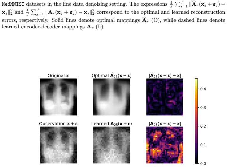
[Figure 4 caption] The sentence 'with low.' appears incomplete; it should continue with a description of the error magnitude.

Circularity Check

0 steps flagged · score 2.0 of 10

Central closed-form derivations are not circular; SWE validation has validity issues (model misspecification and full-data rank selection) but no equation-level circularity.

full rationale

The paper's main results (Theorems 2 and 4) are derived from a well-defined Bayes-risk minimization by completing the square and applying the external Friedland-Torokhti rank-constrained approximation theorem [55] (quoted as Theorem 1). The optimal mappings are not assumed as inputs; they are consequences of the objective. The special cases (autoencoding, denoising) follow by substituting F=I and recover classical PCA/Wiener results, which the paper explicitly frames as links to prior literature rather than new predictions. Self-citations [36,37,73] are used as motivation and context, not as load-bearing steps in the proofs. The main caveats are empirical, not circular: in Section 5.3 the paper states 'Although we know a priori that the SWEs are nonlinear...' and then approximates E[XY^T] by (1/J)XY^T, which replaces the theorem's identity E[XY^T]=Γ_X F^T with a sample quantity; this is an assumption violation, not a circular derivation. The passage 'Experiments with different values of r demonstrated that the minimal RMSE across the entire dataset was obtained at r ≈ 250' shows rank selection on the full dataset, which biases the reported test comparisons, but again is a data-leakage/validity issue. Because the closed-form theory is self-contained and grounded in an external theorem, no circular step can be exhibited; score 2 reflects minor self-citation presence and these validation caveats.

Assumptions & free parameters 5 free parameters · 6 assumptions · 0 invented entities

The ledger shows the central claim rests on the linear observation model, quadratic loss, and Friedland-Torokhti's external theorem. The free parameters are mostly experimental setup choices; the SWE rank selection is the most concerning because it is tuned on the full dataset.

free parameters (5)

bottleneck rank r = r=250 in SWE (selected by minimizing RMSE over full dataset); r=3 in finance; swept in MedMNIST
The rank constraint is the central user-chosen hyperparameter. In the SWE experiment the value is chosen post hoc on the test set, which can inflate reported performance.
ridge regularization term = 1e-2 in SWE; unspecified 'small' in MedMNIST
Added to empirical second-moment matrices to ensure SPD for Cholesky; affects the computed optimal map though usually mildly.
noise standard deviation s_E = 0.05 in MedMNIST
Sets the noise level in the synthetic observation model; the paper does not vary it.
Gaussian blur kernel width s_F = 1.5 in MedMNIST
Defines the forward operator F in the imaging experiment; chosen by the authors.
financial factor count = 3
Latent dimension for the autoencoder, chosen to match the Fama-French three-factor model; not justified by data.

assumptions (6)

domain assumption Observations follow Y = FX + E with E independent of X and zero-mean, with finite second moments (Eq. 1)
This is the data-generating model throughout Section 4; if it fails, the closed-form Bayes-optimal interpretation breaks.
domain assumption Loss is expected squared l2 error (Bayes risk under quadratic loss)
All theorems minimize E||AX - Y||^2; other losses would give different optimal maps.
standard math Theorem 1 (Friedland-Torokhti) is used as a black box
The paper states Theorem 1 and says 'Proof. See [55].' The entire derivation relies on this external theorem.
standard math Second-moment matrices admit symmetric PSD factorizations Gamma_X = L_X L_X^T with L_X full row rank up to rank(Gamma_X)
Every PSD matrix has such a factorization; used throughout Section 4.
domain assumption In the empirical setting, sample moments consistently estimate population moments
The paper replaces Gamma_X, Gamma_Y, Gamma_X F^T with sample statistics; the claimed optimality is asymptotic or approximate.
domain assumption The inverse problem's optimality relies on the linear forward model: E[XY^T] = Gamma_X F^T
Used in Theorem 4 and in the SWE experiment; if the forward process is nonlinear, the derived map is not necessarily Bayes optimal.

how reviews work

0 comments

Cite this review

Pith. "Pith review of Optimal Linear Baseline Models for Scientific Machine Learning." pith.science (2026). https://pith.science/paper/SRSJXCY3

@misc{pith2026250805831,
  author       = {Pith},
  title        = {Pith review of: Optimal Linear Baseline Models for Scientific Machine Learning},
  year         = {2026},
  howpublished = {\url{https://pith.science/paper/SRSJXCY3}},
  note         = {Machine review of arXiv:2508.05831}
}

read the original abstract

Across scientific domains, a fundamental challenge is to characterize and compute the mappings from underlying physical processes to observed signals and measurements. While nonlinear neural networks have achieved considerable success, they remain theoretically opaque, which hinders adoption in contexts where interpretability is paramount. In contrast, linear neural networks serve as a simple yet effective foundation for gaining insight into these complex relationships. In this work, we develop a unified theoretical framework for analyzing linear encoder-decoder architectures through the lens of Bayes risk minimization for solving data-driven scientific machine learning problems. We derive closed-form, rank-constrained linear and affine linear optimal mappings for forward modeling and inverse recovery tasks. Our results generalize existing formulations by accommodating rank-deficiencies in data, forward operators, and measurement processes. We validate our theoretical results by conducting numerical experiments on datasets from simple biomedical imaging, financial factor analysis, and simulations involving nonlinear fluid dynamics via the shallow water equations. This work provides a robust baseline for understanding and benchmarking learned neural network models for scientific machine learning problems.

Figures

Figures reproduced from arXiv: 2508.05831 by the authors.

**Figure 1.** End-to-end encoder-decoder architecture. The input x is mapped by Ex onto a latent variable z, then decoded by y ≈ Dz + b to obtain a target vector y. The remainder of this paper will focus on such linear (and correspondingly affine linear) encoder-decoders and autoencoders, and their application to scientific ML problem formulations. We note that in the literature, the terms encoder-decoder and autoencoder are oft… view at source ↗

**Figure 2.** Example of the forward end-to-end process on sample 7181 from ChestMNIST. The left image shows the original input x; the center image shows the blurred version Fx after application of the forward operator F; and the right image shows the final observed measurement y = Fx + ε after addition of Gaussian noise ε. 5.1 MedMNIST Study We begin with a basic biomedical imaging example. For this investigation, we focus prima… view at source ↗

**Figure 3.** Average per-sample ℓ2 reconstruction error versus bottleneck rank r across MedMNIST datasets for both forward and inverse end-to-end problems. Left: Forward process, where the goal is to learn a mapping from x to y. The optimal and learned mappings minimize the empirical losses 1 J PJ j=1 ∥Ab F r xj − yj∥ 2 2 and 1 J PJ j=1 ∥AF r xj − yj∥ 2 2, respectively. Right: Inverse process, where the goal is to reconstruct x … view at source ↗

Figures from the paper (7 more)

**Figure 4.** Figure 4: Example reconstruction results from ChestMNIST with bottleneck rank r = 25 for both forward and inverse end-to-end problems. In all cases, the observed measurement is denoted y and the ground truth is x. Top row: Reconstructions using optimal mappings. Left to right: o…

**Figure 5.** Figure 5: Visualization of the four different kinds of initial conditions used in the dataset. Note that the z axis denotes η (m) for the first and fourth columns, u (m/s) for the second and fifth columns and v (m/s) for the others columns. sion of our stock universe. More gener…

**Figure 6.** Figure 6: Example of actual initial conditions, linear model reconstructions, and nonlinear learned model reconstructions for all three variables, for an instance from the out-ofdistribution testing set. 24 [PITH_FULL_IMAGE:figures/full_fig_p024_6.png]

**Figure 7.** Figure 7: Average per-sample ℓ2 reconstruction error versus bottleneck rank r across MedMNIST datasets for the classic noiseless autoencoder problem, where the goal is to learn a rank constrained identity mapping from x to x. The optimal and learned mappings minimize the empiric…

**Figure 8.** Figure 8: Example reconstruction results from ChestMNIST with bottleneck rank r = 25 for the classic linear noiseless autoencoder problem. Top row: Reconstructions using optimal mappings. Left to right: original signal x; optimal reconstruction Ab 25x and corresponding error map…

**Figure 9.** Figure 9: Average per-sample ℓ2 reconstruction error versus bottleneck rank r across MedMNIST datasets in the line data denoising setting. The expressions 1 J PJ j=1 ∥Ab r(xj + εj ) − xj∥ 2 2 and 1 J PJ j=1 ∥Ar(xj + εj ) − xj∥ 2 2 correspond to the optimal and learned reconstruc…

**Figure 10.** Figure 10: Example reconstruction results from ChestMNIST with bottleneck rank r = 25 in the linear data denoising setting. Top row: original ground-truth image x; optimal denoised reconstruction Ab 25(x + ε); and reconstruction error map |Ab 25(x + ε) − x|. Bottom row: noisy ob…

Discussion (0). Sign in to comment.

Reference graph

Works this paper leans on

117 extracted references · 41 canonical work pages

[1]

Deep Learning

Ian Goodfellow et al. Deep Learning. Vol. 1. 2. Cambridge, MA, USA: MIT Press, 2016. url: http: //www.deeplearningbook.org

2016
[2]

Surrogate and reduced-order modeling: a comparison of approaches for large- scale statistical inverse problems

Michalis Frangos et al. “Surrogate and reduced-order modeling: a comparison of approaches for large- scale statistical inverse problems”. In: Large-Scale Inverse Problems and Quantification of Uncertainty (2010), pp. 123–149. doi: 10.1002/9780470685853.ch7

work page doi:10.1002/9780470685853.ch7 2010
[3]

Kernel methods for surrogate modeling

Gabriele Santin, Bernard Haasdonk, et al. “Kernel methods for surrogate modeling”. In: System- and Data-Driven Methods and Algorithms . Vol. 1. De Gruyter, 2021, pp. 311–353. doi: 10.1515/ 9783110498967

2021
[4]

Physics-informed neural networks: a deep learning framework for solving forward and inverse problems involving nonlinear partial differential equations

Maziar Raissi, Paris Perdikaris, and George E Karniadakis. “Physics-informed neural networks: a deep learning framework for solving forward and inverse problems involving nonlinear partial differential equations”. In: Journal of Computational Physics 378 (2019), pp. 686–707. doi: 10.1016/j.jcp. 2018.10.045

doi:10.1016/j.jcp 2019
[5]

Scientific machine learning through physics–informed neural networks: where we are and what’s next

Salvatore Cuomo et al. “Scientific machine learning through physics–informed neural networks: where we are and what’s next”. In: Journal of Scientific Computing 92.3 (2022), p. 88. doi: 10 . 1007 / s10915-022-01939-z

2022
[6]

Deep neural network approach to forward-inverse problems

Hyeontae Jo et al. “Deep neural network approach to forward-inverse problems”. In: Networks and Heterogeneous Media 15.2 (2020), pp. 247–259. issn: 1556-1801. doi: 10.3934/nhm.2020011. 26

work page doi:10.3934/nhm.2020011 2020
[7]

Exact representation and efficient approximations of linear model predictive control laws via HardTanh type deep neural networks

Daniela Lupu and Ion Necoara. “Exact representation and efficient approximations of linear model predictive control laws via HardTanh type deep neural networks”. In: Systems & Control Letters 186 (2024), p. 105742. doi: 10.1016/j.sysconle.2024.105742

work page arXiv 2024
[8]

Inverse Problem Theory and Methods for Model Parameter Estimation

Albert Tarantola. Inverse Problem Theory and Methods for Model Parameter Estimation . Society for Industrial and Applied Mathematics, 2005. doi: 10.1137/1.9780898717921

doi:10.1137/1.9780898717921 2005

Show all 117 references

[9]

Discrete Inverse Problems: Insight and Algorithms

Per Christian Hansen. Discrete Inverse Problems: Insight and Algorithms . Society for Industrial and Applied Mathematics, 2010. doi: 10.1137/1.9780898718836

2010 doi
[10]

Sur les probl` emes aux d´ eriv´ ees partielles et leur signification physique

Jacques Hadamard. “Sur les probl` emes aux d´ eriv´ ees partielles et leur signification physique”. In: Princeton University Bulletin (1902), pp. 49–52

1902
[11]

Richard E. Bellman. Adaptive Control Processes: A Guided Tour . Princeton, NJ, USA: Princeton University Press, 1961. doi: 10.1515/9781400874668

1961 doi
[12]

Solving inverse problems using data-driven models

Simon Arridge et al. “Solving inverse problems using data-driven models”. In: Acta Numerica 28 (2019), pp. 1–174. doi: 10.1017/S0962492919000059

2019 doi
[13]

Modern regularization methods for inverse problems

Martin Benning and Martin Burger. “Modern regularization methods for inverse problems”. In: Acta Numerica 27 (2018), pp. 1–111. doi: 10.1017/S0962492918000016

2018 doi
[14]

Variational regularization in inverse problems and machine learning

Martin Burger. “Variational regularization in inverse problems and machine learning”. In: European Congress of Mathematics . Ed. by Andreja Hudj´ urov´ a et al. Z¨ urich: European Mathematical Society Publishing House, 2021, pp. 253–275. doi: 10.4171/8ECM/01

2021 doi
[15]

Solution paths of variational regularization methods for inverse problems

Leon Bungert and Martin Burger. “Solution paths of variational regularization methods for inverse problems”. In: Inverse Problems 35.10 (2019), p. 105012. doi: 10.1088/1361-6420/ab1d71

2019 doi
[16]

Iterative regularization with a general penalty term-theory and application to L1 and TV regularization

Radu Ioan Bot ¸ and Torsten Hein. “Iterative regularization with a general penalty term-theory and application to L1 and TV regularization”. In: Inverse Problems 28.10 (2012), p. 104010. doi: 10. 1088/0266-5611/28/10/104010

2012
[17]

Iterative total variation schemes for nonlinear inverse prob- lems

Markus Bachmayr and Martin Burger. “Iterative total variation schemes for nonlinear inverse prob- lems”. In: Inverse Problems 25.10 (2009), p. 105004. doi: 10.1088/0266-5611/25/10/105004

2009 doi
[18]

Empirical Bayesian regularization of the inverse acoustic problem

Antonio Pereira, J´ erˆ ome Antoni, and Quentin Leclere. “Empirical Bayesian regularization of the inverse acoustic problem”. In: Applied Acoustics 97 (2015), pp. 11–29. doi: 10.1016/j.apacoust. 2015.03.008

2015 doi
[19]

Inverse problems: from regularization to Bayesian inference

Daniela Calvetti and Erkki Somersalo. “Inverse problems: from regularization to Bayesian inference”. In: Wiley Interdisciplinary Reviews: Computational Statistics 10.3 (2018), e1427. doi: 10.1002/wics. 1427

2018 doi
[20]

Deep learning techniques for inverse problems in imaging

Gregory Ongie et al. “Deep learning techniques for inverse problems in imaging”. In: IEEE Journal on Selected Areas in Information Theory 1.1 (2020), pp. 39–56. doi: 10.1109/JSAIT.2020.2991563

2020
[21]

Deep learning methods for inverse problems

Shima Kamyab et al. “Deep learning methods for inverse problems”. In: PeerJ Computer Science 8 (2022), e951. doi: 10.7717/peerj-cs.951

2022 doi
[22]

Learning regularization parameters of inverse problems via deep neural networks

Babak Maboudi Afkham, Julianne Chung, and Matthias Chung. “Learning regularization parameters of inverse problems via deep neural networks”. In: Inverse Problems 37.10 (2021), p. 105017. doi: 10.1088/1361-6420/ac245d

2021 doi
[23]

Deep convolutional neural network for inverse problems in imaging

Kyong Hwan Jin et al. “Deep convolutional neural network for inverse problems in imaging”. In: IEEE Transactions on Image Processing 26.9 (2017), pp. 4509–4522. doi: 10.1109/TIP.2017.2713099

2017
[24]

Solving inverse problems in medical imaging with score-based generative models

Yang Song et al. “Solving inverse problems in medical imaging with score-based generative models”. In: arXiv preprint arXiv:2111.08005 (2021). url: https://arxiv.org/abs/2111.08005

2021 arXiv
[25]

Convolutional neural networks for inverse problems in imaging: a review

Michael T. McCann, Kyong Hwan Jin, and Michael Unser. “Convolutional neural networks for inverse problems in imaging: a review”. In: IEEE Signal Processing Magazine 34.6 (2017), pp. 85–95. doi: 10.1109/MSP.2017.2739299. 27

2017
[26]

Using deep neural networks for inverse problems in imaging: beyond analytical methods

Alice Lucas et al. “Using deep neural networks for inverse problems in imaging: beyond analytical methods”. In: IEEE Signal Processing Magazine 35.1 (2018), pp. 20–36. doi: 10.1109/MSP.2017. 2760358

2018 doi
[27]

Deep magnetic resonance image reconstruction: inverse problems meet neural networks

Dong Liang et al. “Deep magnetic resonance image reconstruction: inverse problems meet neural networks”. In: IEEE Signal Processing Magazine 37.1 (2020), pp. 141–151. doi: 10.1109/MSP.2019. 2950557

2020 doi
[28]

Interpretation of inaccurate, insufficient and inconsistent data

David D. Jackson. “Interpretation of inaccurate, insufficient and inconsistent data”. In: Geophysical Journal International 28.2 (1972), pp. 97–109. doi: 10.1111/j.1365-246X.1972.tb06115.x

1972 doi
[29]

An application of the Wiener-Kolmogorov smoothing theory to matrix inversion

Manus Foster. “An application of the Wiener-Kolmogorov smoothing theory to matrix inversion”. In: Journal of the Society for Industrial and Applied Mathematics 9.3 (1961), pp. 387–392. doi: https://doi.org/10.1137/0109031

1961 doi
[30]

Steven M. Kay. Fundamentals of Statistical Signal Processing: Estimation Theory . River, NJ, USA: Prentice-Hall, Inc., 1993. doi: 10.5555/151045

1993 doi
[31]

Extrapolation, Interpolation, and Smoothing of Stationary Time Series: with Engi- neering Applications

Norbert Wiener. Extrapolation, Interpolation, and Smoothing of Stationary Time Series: with Engi- neering Applications. Cambridge, MA, USA: The MIT Press, Aug. 1949. doi: 10.7551/mitpress/ 2946.001.0001

1949 doi
[32]

Reduced-Rank Regression for the Multivariate Linear Model

Alan Julian Izenman. “Reduced-Rank Regression for the Multivariate Linear Model”. In: Journal of Multivariate Analysis 5.2 (1975), pp. 248–264. doi: 10.1016/0047-259X(75)90042-1

1975 doi
[33]

The Bayesian approach to inverse problems

Masoumeh Dashti and Andrew M. Stuart. “The Bayesian approach to inverse problems”. In: Handbook of Uncertainty Quantification. Ed. by Roger Ghanem, David Higdon, and Houman Owhadi. Springer International Publishing, 2017, pp. 311–428. doi: 10.1007/978-3-319-12385-1_7

2017 doi
[34]

Wiley, 2008

J´ erˆ ome Idier.Bayesian Approach to Inverse Problems . Wiley, 2008. doi: 10.1002/9780470611197

2008 doi
[35]

Inverse problems: a Bayesian perspective

Andrew M. Stuart. “Inverse problems: a Bayesian perspective”. In: Acta Numerica 19 (2010), pp. 451–

2010
[36]

A paired autoencoder framework for inverse problems via Bayes risk minimization

Emma Hart, Julianne Chung, and Matthias Chung. “A paired autoencoder framework for inverse problems via Bayes risk minimization”. In: arXiv preprint arXiv:2501.14636 (2025). url: https : //arxiv.org/abs/2501.14636

2025 arXiv
[37]

Paired autoencoders for likelihood-free estimation in inverse problems

Matthias Chung et al. “Paired autoencoders for likelihood-free estimation in inverse problems”. In: Machine Learning: Science and Technology 5.4 (2024), p. 045055. doi: 10.1088/2632-2153/ad95dd

2024 doi
[38]

Optimal regularized low rank inverse approximation

Julianne Chung, Matthias Chung, and Dianne P. O’Leary. “Optimal regularized low rank inverse approximation”. In: Linear Algebra and its Applications 468 (2015), pp. 260–269. doi: 10.1016/j. laa.2014.07.024

2015 doi
[39]

Optimal low-rank approximations of Bayesian linear inverse problems

Alessio Spantini et al. “Optimal low-rank approximations of Bayesian linear inverse problems”. In: SIAM Journal on Scientific Computing 37.6 (2015), A2451–A2487. doi: 10.1137/140977308

2015 doi
[40]

Solving Bayesian inverse problems via variational autoencoders

Hwan Goh et al. “Solving Bayesian inverse problems via variational autoencoders”. In: Proceedings of the 2nd Mathematical and Scientific Machine Learning Conference . Ed. by Joan Bruna, Jan Hes- thaven, and Lenka Zdeborova. Vol. 145. Proceedings of Machine Learning Research. P...

2022
[41]

Why are big data matrices approximately low rank?

Madeleine Udell and Alex Townsend. “Why are big data matrices approximately low rank?” In: SIAM Journal on Mathematics of Data Science 1.1 (2019), pp. 144–160. doi: doi.org/10.1137/ 18M1183480

2019
[42]

Autoencoders and their applications in machine learning: a survey

Kamal Berahmand et al. “Autoencoders and their applications in machine learning: a survey”. In: Artificial Intelligence Review 57.2 (2024), p. 28. doi: doi.org/10.1007/s10462-023-10662-6

2024 doi
[43]

Medical image denoising using convolutional denoising autoencoders

Lovedeep Gondara. “Medical image denoising using convolutional denoising autoencoders”. In: 2016 IEEE 16th International Conference on Data Mining Workshops (ICDMW) . IEEE. 2016, pp. 241–

2016
[44]

Stacked convolutional auto-encoders for hierarchical feature extraction

Jonathan Masci et al. “Stacked convolutional auto-encoders for hierarchical feature extraction”. In: International Conference on Artificial Neural Networks . Springer. 2011, pp. 52–59

2011
[45]

Multilayer feedforward networks are uni- versal approximators

Kurt Hornik, Maxwell Stinchcombe, and Halbert White. “Multilayer feedforward networks are uni- versal approximators”. In: Neural Networks 2.5 (1989), pp. 359–366. doi: 10.1016/0893-6080(89) 90020-8

1989 doi
[46]

The mythos of model interpretability: in machine learning, the concept of inter- pretability is both important and slippery

Zachary C Lipton. “The mythos of model interpretability: in machine learning, the concept of inter- pretability is both important and slippery”. In: Queue 16.3 (2018), pp. 31–57. doi: 0.1145/3236386. 3241340

2018
[47]

A survey on neural network interpretability

Yu Zhang et al. “A survey on neural network interpretability”. In: IEEE Transactions on Emerging Topics in Computational Intelligence 5.5 (2021), pp. 726–742. doi: 10.1109/TETCI.2021.3100641

2021
[48]

Neural networks and principal component analysis: learning from examples without local minima

Pierre Baldi and Kurt Hornik. “Neural networks and principal component analysis: learning from examples without local minima”. In: Neural Networks 2.1 (1989), pp. 53–58. doi: 10.1016/0893- 6080(89)90014-2

1989 doi
[49]

Auto-association by multilayer perceptrons and singular value decompo- sition

H. Bourlard and Y. Kamp. “Auto-association by multilayer perceptrons and singular value decompo- sition”. In: Biological Cybernetics 59.4-5 (1988), pp. 291–294. doi: 10.1007/bf00332918

1988 doi
[50]

From principal subspaces to principal components with linear autoencoders

Elad Plaut. “From principal subspaces to principal components with linear autoencoders”. In: arXiv preprint: arXiv:1804.10253 (2018). url: https://arxiv.org/abs/1804.10253

2018 arXiv
[51]

Regularized linear autoencoders recover the principal components, eventually

Xuchan Bao et al. “Regularized linear autoencoders recover the principal components, eventually”. In: Advances in Neural Information Processing Systems. Vol. 33. Curran Associates, Inc., 2020, pp. 6971– 6981

2020
[52]

The approximation of one matrix by another of lower rank

Carl Eckart and Gale Young. “The approximation of one matrix by another of lower rank”. In: Psychometrika 1.3 (1936), pp. 211–218

1936
[53]

Symmetric gauge functions and unitarily invariant norms

Leon Mirsky. “Symmetric gauge functions and unitarily invariant norms”. In: The Quarterly Journal of Mathematics 11.1 (1960), pp. 50–59. doi: 10.1093/qmath/11.1.50

1960 doi
[54]

Zur theorie der linearen und nichtlinearen integralgleichungen

Erhard Schmidt. “Zur theorie der linearen und nichtlinearen integralgleichungen”. In: Mathematische Annalen 63.4 (1907), pp. 433–476. doi: 10.1007/BF01449770

1907 doi
[55]

Generalized rank-constrained matrix approximations

Shmuel Friedland and Anatoli Torokhti. “Generalized rank-constrained matrix approximations”. In: SIAM Journal on Matrix Analysis and Applications 29.2 (2007), pp. 656–659. doi: 10 . 1137 / 06065551

2007
[56]

Finding structure with randomness: probabilistic algo- rithms for constructing approximate matrix decompositions

N. Halko, P. G. Martinsson, and J. A. Tropp. “Finding structure with randomness: probabilistic algo- rithms for constructing approximate matrix decompositions”. In: SIAM Review 53.2 (2011), pp. 217–

2011
[57]

Near-optimal column-based matrix reconstruction

Christos Boutsidis, Petros Drineas, and Malik Magdon-Ismail. “Near-optimal column-based matrix reconstruction”. In: SIAM Journal on Computing 43.2 (2014), pp. 687–717. doi: 10.1137/12086755X

2014 doi
[58]

Dimensionality reduction for k-means clustering and low rank approxi- mation

Michael B. Cohen et al. “Dimensionality reduction for k-means clustering and low rank approxi- mation”. In: Proceedings of the Forty-Seventh Annual ACM Symposium on Theory of Computing . STOC ’15. Portland, Oregon, USA: Association for Computing Machinery, 2015, pp. 163–172. d...

2015
[59]

Low-rank matrix approximation with manifold regularization

Zhenyue Zhang and Keke Zhao. “Low-rank matrix approximation with manifold regularization”. In: IEEE Transactions on Pattern Analysis and Machine Intelligence 35.7 (July 2013), pp. 1717–1729. doi: 10.1109/tpami.2012.274

2013 doi
[60]

Subspace-orbit randomized decomposi- tion for low-rank matrix approximations

Maboud Farzaneh Kaloorazi and Rodrigo C. de Lamare. “Subspace-orbit randomized decomposi- tion for low-rank matrix approximations”. In: IEEE Transactions on Signal Processing 66.16 (2018), pp. 4409–4424. doi: 10.1109/TSP.2018.2853137

2018
[61]

Dimensionality reduction strategy based on auto-encoder

Yasi Wang et al. “Dimensionality reduction strategy based on auto-encoder”. In: Proceedings of the 7th International Conference on Internet Multimedia Computing and Service . Zhangjiajie Hunan China: ACM, Aug. 2015, pp. 1–4. doi: 10.1145/2808492.2808555. 29

2015
[62]

Rank reduction autoencoders

Jad Mounayer et al. “Rank reduction autoencoders”. In: arXiv preprint: arXiv:2405.13980 (2025). url: https://arxiv.org/abs/2405.13980

2025 arXiv
[63]

Learning-based low-rank approximations

Piotr Indyk, Ali Vakilian, and Yang Yuan. “Learning-based low-rank approximations”. In: Proceedings of the 33rd International Conference on Neural Information Processing Systems. Red Hook, NY, USA: Curran Associates Inc., 2019. doi: 10.5555/3454287.3454952

2019
[64]

Sparse Bayesian methods for low-rank matrix estimation

S. Derin Babacan et al. “Sparse Bayesian methods for low-rank matrix estimation”. In: IEEE Trans- actions on Signal Processing 60.8 (2012), pp. 3964–3977. doi: 10.1109/tsp.2012.2197748

2012
[65]

Learning low-rank latent spaces with simple deterministic autoencoder: theoretical and empirical insights

Alokendu Mazumder et al. “Learning low-rank latent spaces with simple deterministic autoencoder: theoretical and empirical insights”. In: 2024 IEEE/CVF Winter Conference on Applications of Com- puter Vision (WACV) . Waikoloa, HI, USA: IEEE, 2024, pp. 2839–2848. doi: 10.1109/wa...

2024
[66]

Bayes and empirical Bayes methods for data analysis

Bradley P. Carlin and Thomas A. Louis. “Bayes and empirical Bayes methods for data analysis”. In: Statistics and Computing 7.2 (June 1997), pp. 153–154. doi: 10.1023/A:1018577817064

1997 doi
[67]

Computing optimal low-rank matrix approximations for image processing

Julianne Chung and Matthias Chung. “Computing optimal low-rank matrix approximations for image processing”. In: 2013 Asilomar Conference on Signals, Systems and Computers . IEEE. 2013, pp. 670–

2013
[68]

Optimal regularized inverse matrices for inverse problems

Julianne Chung and Matthias Chung. “Optimal regularized inverse matrices for inverse problems”. In: SIAM Journal on Matrix Analysis and Applications 38.2 (2017), pp. 458–477. doi: 10 . 1137 / 16M1066531

2017
[69]

An efficient approach for computing optimal low-rank regu- larized inverse matrices

Julianne Chung and Matthias Chung. “An efficient approach for computing optimal low-rank regu- larized inverse matrices”. In: Inverse Problems 30.11 (2014), p. 114009. doi: 10.1088/0266-5611/ 30/11/114009

2014 doi
[70]

Auto-encoding variational Bayes

Diederik P. Kingma and Max Welling. “Auto-encoding variational Bayes”. In: arXiv preprint arXiv:1312.6114 (2013). url: https://arxiv.org/abs/1312.6114

2013 arXiv
[71]

On the reciprocal of the general algebraic matrix

Eliakim H Moore. “On the reciprocal of the general algebraic matrix”. In: Bulletin of the American Mathematical Society 26 (1920), pp. 294–295

1920
[72]

A generalized inverse for matrices

Roger Penrose. “A generalized inverse for matrices”. In: Mathematical Proceedings of the Cambridge Philosophical Society . Vol. 51. 3. Cambridge University Press. 1955, pp. 406–413. doi: 10 . 1017 / S0305004100030401

1955
[73]

Good things come in pairs: paired autoencoders for inverse problems

Matthias Chung, Bas Peters, and Michael Solomon. “Good things come in pairs: paired autoencoders for inverse problems”. In: arXiv preprint: arXiv:2505.06549 (2025). url: https://www.arxiv.org/ abs/2505.06549

2025 arXiv
[74]

The Elements of Statistical Learning

Trevor Hastie, Robert Tibshirani, and Jerome Friedman. The Elements of Statistical Learning . New York, NY,USA: Springer, 2009. doi: 10.1007/978-0-387-84858-7

2009 doi
[75]

Williams and Carl E

Christopher K.I. Williams and Carl E. Rasmussen. Gaussian Processes for Machine Learning. Vol. 2
[76]

MedMNIST v2-a large-scale lightweight benchmark for 2D and 3D biomedical image classification

Jiancheng Yang et al. “MedMNIST v2-a large-scale lightweight benchmark for 2D and 3D biomedical image classification”. In: Scientific Data 10.1 (2023), p. 41

2023
[77]

Annotated high-throughput mi- croscopy image sets for validation

Vebjorn Ljosa, Katherine L Sokolnicki, and Anne E Carpenter. “Annotated high-throughput mi- croscopy image sets for validation”. In: Nature Methods 9.7 (2012), pp. 637–637

2012
[78]

ChestX-ray8: hospital-scale chest x-ray database and benchmarks on weakly-supervised classification and localization of common thorax diseases

Xiaosong Wang, Yifan Peng, et al. “ChestX-ray8: hospital-scale chest x-ray database and benchmarks on weakly-supervised classification and localization of common thorax diseases”. In: CVPR. 2017, pp. 3462–3471

2017
[79]

The liver tumor segmentation benchmark (LiTS)

Patrick Bilic, Patrick Ferdinand Christ, et al. “The liver tumor segmentation benchmark (LiTS)”. In: CoRR abs/1901.04056 (2019). arXiv: 1901.04056. 30

1901 arXiv
[80]

Cambridge, MA, USA: MIT Press, 2006

2006
[81]

Adam: A method for stochastic optimization

Diederik P Kingma and Jimmy Ba. “Adam: A method for stochastic optimization”. In: arXiv preprint arXiv:1412.6980 (2014). url: https://arxiv.org/abs/1412.6980

2014 arXiv
[82]

Common risk factors in the returns on stocks and bonds

Eugene F. Fama and Kenneth R. French. “Common risk factors in the returns on stocks and bonds”. In: Journal of Financial Economics 33.1 (1993), pp. 3–56. doi: 10.1016/0304-405X(93)90023-5

1993 doi
[83]

Capital asset prices: a theory of market equilibrium under conditions of risk

William F. Sharpe. “Capital asset prices: a theory of market equilibrium under conditions of risk”. In: The Journal of Finance 19.3 (1964), pp. 425–442. doi: 10.1111/j.1540-6261.1964.tb02865.x

1964
[84]

The cross-section of expected stock returns

Eugene F. Fama and Kenneth R. French. “The cross-section of expected stock returns”. In: The Journal of Finance 47.2 (1992), pp. 427–465. doi: 10.1111/j.1540-6261.1992.tb04398.x

1992
[85]

Efficient multiple organ localization in CT image using 3D region proposal network

X. Xu, F. Zhou, et al. “Efficient multiple organ localization in CT image using 3D region proposal network”. In: IEEE Transactions on Medical Imaging 38.8 (2019), pp. 1885–1898

2019
[86]

Volatility clustering and market structure: a volatility factor model

Siddharth Verma, Raffaello Buonocore, and Tiziana Di Matteo. “Volatility clustering and market structure: a volatility factor model”. In: arXiv preprint arXiv:1712.02138 (2017). url: https : / / arxiv.org/abs/1712.02138

2017 arXiv
[87]

The arbitrage theory of capital asset pricing

Steven A. Ross. “The arbitrage theory of capital asset pricing”. In: Journal of Economic Theory 13.3 (1976), pp. 341–360. doi: 10.1016/0022-0531(76)90046-6

1976 doi
[88]

yfinance: fownload market data from Yahoo! Finance’s API

Ran Aroussi. yfinance: fownload market data from Yahoo! Finance’s API . https://github.com/ ranaroussi/yfinance. Accessed: 2025-07-15. 2015

2025
[89]

Quant GANs: deep generation of financial time series

Magnus Wiese et al. “Quant GANs: deep generation of financial time series”. In: Quantitative Finance 20.9 (2020), pp. 1419–1440. doi: 10.1080/14697688.2020.1730426

2020
[90]

Principal component analysis

Ian Jolliffe. “Principal component analysis”. In: International Encyclopedia of Statistical Science . Ed. by Miodrag Lovric. Berlin, Heidelberg: Springer Berlin Heidelberg, 2011, pp. 1094–1096. doi: 10.1007/978-3-642-04898-2_455

2011 doi
[91]

The Varimax criterion for analytic rotation in factor analysis

Henry F. Kaiser. “The Varimax criterion for analytic rotation in factor analysis”. In: Psychometrika 23.3 (1958), pp. 187–200. doi: 10.1007/BF02289233

1958 doi
[92]

A matrix formulation of Kaiser’s Varimax criterion

Richard J. Sherin. “A matrix formulation of Kaiser’s Varimax criterion”. In: Psychometrika 31.4 (1966), pp. 535–538. doi: 10.1007/BF02289522

1966 doi
[93]

An overview of analytic rotation in exploratory factor analysis

Michael W. Browne. “An overview of analytic rotation in exploratory factor analysis”. In: Multivariate Behavioral Research 36.1 (2001), pp. 111–150

2001
[94]

Fama and Kenneth R

Eugene F. Fama and Kenneth R. French. Kenneth R. French data library . https : / / mba . tuck . dartmouth.edu/pages/faculty/ken.french/data_library.html. Accessed: 2025-08-01. 2025

2025
[95]

Campbell, Andrew W

John Y. Campbell, Andrew W. Lo, and A. Craig MacKinlay. The Econometrics of Financial Markets . Princeton University Press, 1997. doi: 10.2307/j.ctt7skm5

1997 doi
[96]

Brockwell and Richard A

Peter J. Brockwell and Richard A. Davis. Introduction to Time Series and Forecasting. Springer, 2016. doi: 10.1007/978-3-319-29854-2

2016 doi
[97]

Generalized autoregressive conditional heteroskedasticity

Tim Bollerslev. “Generalized autoregressive conditional heteroskedasticity”. In: Journal of Economet- rics 31.3 (1986), pp. 307–327. doi: 10.1016/0304-4076(86)90063-1

1986 doi
[98]

Unsupervised alignment of embeddings with Wasserstein Procrustes

Edouard Grave, Armand Joulin, and Quentin Berthet. “Unsupervised alignment of embeddings with Wasserstein Procrustes”. In: The 22nd International Conference on Artificial Intelligence and Statis- tics. PMLR. 2019, pp. 1880–1890

2019
[99]

A mechanism for producing aligned latent spaces with autoen- coders

Prachi Jain and Soumen Chakrabarti. “A mechanism for producing aligned latent spaces with autoen- coders”. In: arXiv preprint arXiv:2106.15456 (2021). url: https://arxiv.org/abs/2106.15456

2021 arXiv
[100]

A value for n-person games

LLoyd S. Shapley. “A value for n-person games”. In: Contributions to the Theory of Games, Volume II. Ed. by Harold William Kuhn and Albert William Tucker. Princeton: Princeton University Press, 1953, pp. 307–318. doi: doi:10.1515/9781400881970-018

1953 doi
[101]

Hyperalignment: modeling shared information encoded in idiosyncratic cortical topographies

James V. Haxby et al. “Hyperalignment: modeling shared information encoded in idiosyncratic cortical topographies”. In: eLife 9 (2020), e56601. doi: 10.7554/eLife.56601

2020 doi
[102]

Geoffrey K. Vallis. Atmospheric and Oceanic Fluid Dynamics. 2nd. Cambridge University Press, 2017. doi: 10.1017/9781107588417

2017 doi
[103]

¨Uber die partiellen differenzengleichungen der mathematischen physik

Richard Courant, Kurt Friedrichs, and Hans Lewy. “ ¨Uber die partiellen differenzengleichungen der mathematischen physik”. In:Mathematische Annalen 100.1 (1928), pp. 32–74.doi: 10.1007/BF01448839. A Special Case MedMNIST Figures In this appendix we provide some analysis on the...

1928 doi
[105]

A common, high-dimensional model of the representational space in human ventral temporal cortex

James V. Haxby et al. “A common, high-dimensional model of the representational space in human ventral temporal cortex”. In: Neuron 72.2 (2011), pp. 404–416. 31

2011
[109]

R denotes the expected rate of return of an asset
[110]

Rf denotes the risk-free return rate or the theoretical return of a zero-risk investment, constant across all assets
[111]

The Market Excess factor(Market) quantifies the extent at which a market portfolio’s return exceeds Rf
[112]

The Size factor (SMB) measures the extent at which small cap stocks outperform large cap stocks
[113]

The Value factor (HML) measures the extent at which value stocks outperform growth stocks
[114]

The α parameter denotes the mean excess return of not explained by the three Fama-French factors, which varies across assets
[115]

These parameters are usually used for calculating R, and therefore are not a part of this work

γ1, γ2, γ3 are model parameters that vary by asset. These parameters are usually used for calculating R, and therefore are not a part of this work. 35 B.3 Notable Processes
[116]

The time series can be described by the following: Xt = βXt−1 + ϵ2 t where Xt is a stationary series, β is some correlation factor, and ϵ2 t ∼ N(0, υ2) is white noise [96]

AR(1), also known as an Autoregressive Process of Order 1, assumes that each term in a time series depends linearly on the preceding value and some error term. The time series can be described by the following: Xt = βXt−1 + ϵ2 t where Xt is a stationary series, β is some corre...
[117]

Additional parameters were initialized as ω = 0.01, α = 0.1, and β = 0.85 as these values resemble those of the U.S

GARCH(1 , 1) generates a time series Xt = υ2 t for the volatility squared (variance) of a time series, which can be described by the following: υ2 t = ω + αϵ2 t−1 + βυ 2 t−1 where υ2 t represents the variance,ϵt represents residual error from the most recent estimate,ω represe...
[246]

doi: 10.1109/ICDMW.2016.0041. 28

2016
[288]

doi: 10.1137/090771806

doi
[559]

doi: 10.1017/S0962492910000061

doi
[674]

doi: 10.1109/ACSSC.2013.6810366

2013

Pith tools

Reviewed August 5, 2026 · model on record in the stance chip above.

[1] [1]

Deep Learning

Ian Goodfellow et al. Deep Learning. Vol. 1. 2. Cambridge, MA, USA: MIT Press, 2016. url: http: //www.deeplearningbook.org

2016

[2] [2]

Surrogate and reduced-order modeling: a comparison of approaches for large- scale statistical inverse problems

Michalis Frangos et al. “Surrogate and reduced-order modeling: a comparison of approaches for large- scale statistical inverse problems”. In: Large-Scale Inverse Problems and Quantification of Uncertainty (2010), pp. 123–149. doi: 10.1002/9780470685853.ch7

work page doi:10.1002/9780470685853.ch7 2010

[3] [3]

Kernel methods for surrogate modeling

Gabriele Santin, Bernard Haasdonk, et al. “Kernel methods for surrogate modeling”. In: System- and Data-Driven Methods and Algorithms . Vol. 1. De Gruyter, 2021, pp. 311–353. doi: 10.1515/ 9783110498967

2021

[4] [4]

Physics-informed neural networks: a deep learning framework for solving forward and inverse problems involving nonlinear partial differential equations

Maziar Raissi, Paris Perdikaris, and George E Karniadakis. “Physics-informed neural networks: a deep learning framework for solving forward and inverse problems involving nonlinear partial differential equations”. In: Journal of Computational Physics 378 (2019), pp. 686–707. doi: 10.1016/j.jcp. 2018.10.045

doi:10.1016/j.jcp 2019

[5] [5]

Scientific machine learning through physics–informed neural networks: where we are and what’s next

Salvatore Cuomo et al. “Scientific machine learning through physics–informed neural networks: where we are and what’s next”. In: Journal of Scientific Computing 92.3 (2022), p. 88. doi: 10 . 1007 / s10915-022-01939-z

2022

[6] [6]

Deep neural network approach to forward-inverse problems

Hyeontae Jo et al. “Deep neural network approach to forward-inverse problems”. In: Networks and Heterogeneous Media 15.2 (2020), pp. 247–259. issn: 1556-1801. doi: 10.3934/nhm.2020011. 26

work page doi:10.3934/nhm.2020011 2020

[7] [7]

Exact representation and efficient approximations of linear model predictive control laws via HardTanh type deep neural networks

Daniela Lupu and Ion Necoara. “Exact representation and efficient approximations of linear model predictive control laws via HardTanh type deep neural networks”. In: Systems & Control Letters 186 (2024), p. 105742. doi: 10.1016/j.sysconle.2024.105742

work page arXiv 2024

[8] [8]

Inverse Problem Theory and Methods for Model Parameter Estimation

Albert Tarantola. Inverse Problem Theory and Methods for Model Parameter Estimation . Society for Industrial and Applied Mathematics, 2005. doi: 10.1137/1.9780898717921

doi:10.1137/1.9780898717921 2005