REVIEW 3 major objections 5 minor 3 references
Robust Data Interpretation for Perturbed Nulling Interferometers via Proper Handling of Correlated Errors
T0 review · 3 major / 5 minor · reviewed 2026-08-05 · deepseek-v4-flash
Pith's one-line read Correlated instrumental noise in nulling interferometers can be tamed by whitening data against the full error covariance, which restores valid detection statistics and sharpens the extracted planetary spectrum.
desk verdict Useful framework and open-source simulators for nulling interferometry, but the detection-statistic calibration is off because temporal correlations are not whitened and the stated chi-square degrees of freedom omit the time axis. read the letter →
The pith
A machine-rendered reading of the paper's core claim, the machinery that carries it, and where it could break.
The reading
What carries the argument
The load-bearing object is the ZCA whitening transform W = Sigma^(-1/2), where Sigma is the instrumental error covariance estimated from a reference-star observation (Eq. 21). Multiplying data and model by W converts the correlated noise model epsilon' ~ N(0, Sigma) into white noise epsilon ~ N(0, I), so the two detection statistics, the Neyman-Pearson test T_NP = y^T x and the energy detector T_ED = y^T y, acquire their textbook normal and chi-square distributions under H0 and H1. The second mechanism is the numerical maximum-likelihood signal extraction (Levenberg-Marquardt), whose inverse Hessian, evaluated at the best-fit SED and position, provides the spectral covariance that carries un
What would settle it
In a simulated observation where the reference-star covariance used for whitening is deliberately mismatched (for example, a calibrator with 10% different flux or a different rotation phase), the empirical null-hypothesis distributions of T_NP and T_ED should depart measurably from the predicted N(0, x^T x) and chi-square forms; alternatively, whitening with a covariance that includes a bright planet's own signal should visibly suppress or distort the planetary signature in the correlation map.
Extended reading notes
Core claim
The paper's central claim is that whitening against the full instrumental error covariance, not just its diagonal variances, is required for valid hypothesis testing and improves characterization. In a simulated reference observation of an Earth twin around a Sun twin at 10 pc with a double Bracewell nuller, whitened data reproduce the ideal-instrument benchmark: clean planetary peak in correlation maps, detection statistics following predicted Gaussian and chi-square distributions under the null hypothesis, and largely vanished short-wavelength systematics. The inverse Hessian of the whitened maximum-likelihood fit also supplies the spectral covariance of the extracted SED, including SED-po
Load-bearing premise
The whitening procedure assumes an accurate estimate of the instrumental error covariance, obtained in this paper from an ideal reference star identical in properties to the science target; a real calibrator with a different brightness, spectral shape, or perturbation state would leave the whitened data partially correlated and shift the detection statistics off their calibrated distributions.
Editorial extensions
If this is right
- Detection claims can rest on calibrated false-alarm probabilities: after whitening, T_NP and T_ED follow their predicted distributions, so the ad hoc S/N >= 7 margin used in earlier LIFE studies is no longer needed under ideal-instrument assumptions.
- A moderately perturbed instrument (0.1% amplitude, 1.5 nm piston, 0.001 rad polarization) performs close to an ideal one in both detection and SED extraction once whitening is applied.
- Stronger perturbations mainly degrade characterization below ~10 microns, the wavelength region where methane absorption signatures lie, identifying which technical requirements actually drive mission performance.
- The extracted planetary spectrum is accompanied by a full spectral covariance, including SED-position correlations, which can be propagated into atmospheric retrievals that previously assumed independent wavelength bins.
- The open-source tools PHRINGE and LIFEsimMC, with their export to the NIFITS data standard, make the framework usable for requirement derivation and future nulling-data processing pipelines.
Reading between the lines
- The same covariance-whitening prescription transfers to other high-contrast observing modes (coronagraphy, kernel-phase, ground-based nullers), where it could replace empirical speckle or stellar-leakage subtraction with a statistically characterized decorrelation step.
- If the calibrator star is not identical to the target, whitening is only approximate; a natural stress test is to propagate an uncertainty or bias in Sigma (such as the flux-ratio scaling in Eq. 36) and check how the false-alarm calibration degrades.
- Because the Hessian-based spectral covariance includes SED-position correlations, retrievals on multiplanet systems may need joint covariance models capturing inter-spectrum correlations, an extension the paper only flags.
- An internal calibration laser, suggested as future work, could make on-sky covariance estimation feasible without a perfect reference star; demonstrating it would settle the framework's practical applicability to real observations.
Editorial analysis
A structured set of objections, weighed in public.
Referee Report
Summary. The paper develops a simulation and analysis framework for nulling interferometry in the presence of correlated instrumental errors. It introduces PHRINGE, a GPU-accelerated synthetic data generator, and LIFEsimMC, an end-to-end Monte Carlo simulator, and applies them to an Earth twin around a Sun twin at 10 pc. The analysis pipeline ZCA-whitens the per-wavelength covariance estimated from a calibration star, applies Neyman-Pearson and energy-detector hypothesis tests, and performs maximum-likelihood signal extraction with a Hessian-based spectral covariance estimate. The central claims are that whitening is essential for a correctly calibrated detection metric and that it improves estimates of the planetary SED.
Significance. If the statistical calibration were correct, this would be a useful contribution to the LIFE requirement-derivation process. The paper ships two open-source tools, uses a 500-realization Monte Carlo comparison, and correctly frames the key comparison as full-covariance whitening versus diagonal-only standardization, which avoids the trivial circularity of comparing whitened data with no preprocessing. However, the detection-calibration claim is weakened by a degrees-of-freedom inconsistency in the energy-detector statistic and by the acknowledged neglect of temporal correlations, which means the theoretical false-alarm thresholds in Eqs. (26) and (29) are not valid for the data actually analyzed. The Hessian covariance estimate also appears to contain a factor-2 error. These issues are addressable, and the underlying framework remains valuable.
major comments (3)
- [§3.2.2, Eq. (28); Fig. 9] There is a mismatch between the stated degrees of freedom and the plotted TED statistic. Equation (28) assigns p = ndiff nλ degrees of freedom, but the TED values in Fig. 9 are about 1.10–1.20 × 10^5, which for the Table 1 setup (nλ ≈ 77, nt = 1440, ndiff = 1) implies that the statistic is being computed on the full time-extended vector, i.e., p ≈ ndiff nλ nt. If so, Eq. (28) and the threshold in Eq. (29) are not the ones actually used. Please state explicitly how the nt samples enter TED and TNP, correct the degrees-of-freedom definition, and re-derive the theoretical thresholds accordingly.
- [§3.1 (Eq. 18); §2.3; Fig. 9] The whitening matrix W = Σ_ref^{-1/2} decorrelates wavelength channels within a single time slice; it does not whiten the time axis. The perturbation time series are pink noise with f_low = 1/Prot, so consecutive 600 s DIT samples are correlated. After per-time-slice whitening, the stacked noise vector is not N(0,I), and therefore the theoretical distributions in Eqs. (25) and (28) and the thresholds in Eqs. (26) and (29) are not valid for the data actually analyzed. The paper acknowledges this in Sec. 2.3 and in the Fig. 9 caption, where the empirical TED deviation from theory is attributed to temporal correlations. To support the abstract's claim that whitening is 'essential for a correct interpretation of the detection metric,' please either include temporal covariance in the whitening, model the temporal correlations analytically, or calibrate the thresholds empirically and report th
- [§3.3, Eq. (35)] The factor 2 in \hatΣ_Θ ≈ 2 H_ℓ^{-1} appears inconsistent with the definition of ℓ in Eq. (31). With ℓ = (1/2) Σ r², where r = model − data, the Hessian H_ℓ is asymptotically J^T J, and the MLE covariance under N(0,I) noise is H_ℓ^{-1}, not 2H_ℓ^{-1}. If the intended quantity is the Hessian of the chi-square (Σ r²), then the factor 2 is correct but Eq. (31) should not contain the 1/2. This affects the 1σ SED uncertainties in Fig. 10 and the spectral covariance matrix in Fig. 12; please correct or justify the factor.
minor comments (5)
- [§3.3, Eqs. (30)–(31)] D is defined in Eq. (14) as the unwhitened data cube, but Eqs. (30) and (31) appear to use the whitened data and model. Please clarify the notation, e.g., by explicitly applying the whitening transformation to D and Tp before writing the likelihood.
- [Author contributions] Typo: 'LFIE simMC' should be 'LIFEsimMC'.
- [§5.3] The sentence 'This pattern is similar to the covariance of the planetary signal as shown in Figure 4 (top)' is confusing, because Figure 4 (top) displays counts, not a covariance matrix.
- [Throughout] The software name is written inconsistently as 'LIFE sim', 'LIFEsimMC', and 'LIFE simMC'; please harmonize.
- [§3.3] Minor wording: 'We can rewrite out Equation (23)' should be 'rewrite Equation (23)'.
Circularity Check
Whitening's white-noise outcome is definitional, but the central characterization claims rest on independent Monte Carlo simulations; no damaging circularity.
-
self definitional
[Section 3.1, Eqs. (15)-(20); Section 4 / Fig. 9]
"y′ = x′ + ε′. (15) Here, we make the assumption that, when the model, x′, matches the data, y′, then ε′∼N (0, Σ) ... We resolve this by performing data whitening ... y≡ Σ^{−1/2} y′ ... This leads to a new model of our data, y = x + ε, where now ε ∼ N(0, I)."
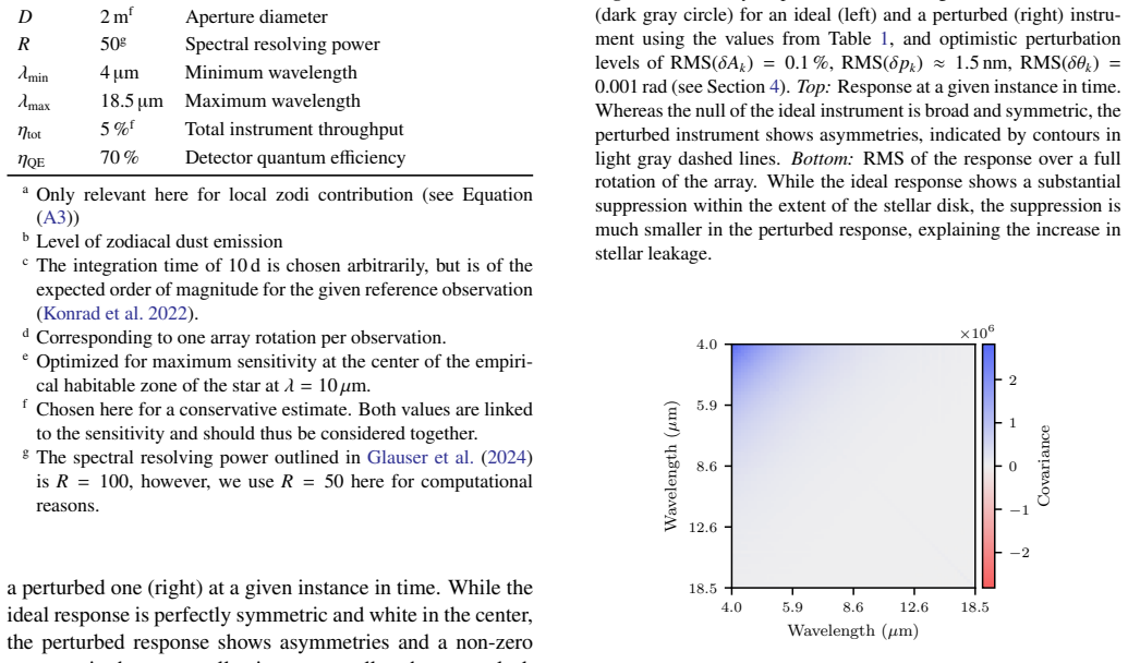
Since ε'~N(0,Σ) is assumed in Eq. (15), applying W=Σ^{−1/2} in Eq. (18) guarantees ε=Wε'~N(0,I) by the affine transformation law for Gaussians. The later demonstration that whitening brings the test statistics 'closer to their theoretical probability density functions' (Fig. 9) is therefore not an independent empirical check of the model: the theoretical N(0,x^T x) and χ²_p laws in Eqs. (25)/(28) are exactly the laws of the transformed variable. The improvement in localization and SED bias over the unwhitened case, however, is an empirical simulation outcome and does not reduce to this identity.
full rationale
The paper's derivation chain is mostly self-contained against external benchmarks and code-reproduced open-source tools (PHRINGE, LIFEsimMC). The core method is standard ZCA whitening (Ceau et al. 2019; Kessy et al. 2018) applied to simulated nulling data, and the claimed improvements in planet localization and SED bias are obtained by Monte Carlo end-to-end simulation, not by fitting the presented results. The one definitional element is that, once ε'~N(0,Σ) is assumed, the whitening transformation W=Σ^{−1/2} makes the transformed noise exactly N(0,I); the post-whitening agreement with Gaussian/χ² theory is thus mathematically forced by the assumed covariance. The paper does not hide this: the covariance is taken from a simulated ideal reference star (Eq. 21) and is explicitly labeled a 'best-case scenario' (Sec. 5.2), and the more informative comparisons against diagonal-only standardization and unwhitened data are empirical. Self-citations (Laugier et al. 2023; Dannert et al. 2025; Huber et al. 2024) are present but not load-bearing: the detection statistics come from external Ceau et al. (2019), and the downstream-optics assumption is also supported by external Lay (2004). No uniqueness theorem is imported from the authors' prior work. The paper's own acknowledged limitations—temporal correlations outside scope and the residual TED mismatch (Sec. 2.3, Fig. 9 caption)—are correctness risks for the calibrated false-alarm rates, not evidence of circularity. Score 3 reflects the mild definitional component while recognizing that the central characterization claims are not forced by the inputs.
Assumptions & free parameters
free parameters (2)
- Instrument perturbation scenario levels (RMS δA, δp, δθ) =
Optimistic: 0.1%, 1.5 nm, 0.001 rad; Pessimistic: 1.0%, 15 nm, 0.010 rad
- Pink noise frequency cutoffs (flow, fhigh) =
flow = 1/Prot ≈ 1.16e-6 Hz, fhigh = 10 kHz
assumptions (5)
- domain assumption Instrumental noise is Gaussian: ε' ~ N(0, Σ)
- domain assumption Calibration star provides exact instrumental error covariance: y'ref = ε'ref and Σref = Cov(y'ref) applies to the science target
- domain assumption Perturbations are pink noise with PSD ∝ 1/ω between flow=1/Prot and fhigh=10 kHz, with amplitude perturbations wavelength-independent and phase perturbations scaling as 1/λ
- domain assumption Perfect spatial filtering by SMF and linear downstream optics, so perturbations reduce to amplitude, phase, and polarization errors at the inputs
- standard math Standard linear algebra: for positive definite Σ, ZCA whitening W = Σ^{-1/2} yields Cov(Wε') = I
Cite this review
Pith. "Pith review of Robust Data Interpretation for Perturbed Nulling Interferometers via Proper Handling of Correlated Errors." pith.science (2026). https://pith.science/paper/GNRTT4GM
@misc{pith2026250815756,
  author       = {Pith},
  title        = {Pith review of: Robust Data Interpretation for Perturbed Nulling Interferometers via Proper Handling of Correlated Errors},
  year         = {2026},
  howpublished = {\url{https://pith.science/paper/GNRTT4GM}},
  note         = {Machine review of arXiv:2508.15756}
}
read the original abstract
The detection and atmospheric characterization of potentially habitable, temperate terrestrial exoplanets using a space-based mid-infrared nulling interferometer is a major goal of contemporary astrophysics. A central part of the analysis of such an instrument are correlated errors arising from perturbations in the system. While previous studies have often treated their effects in a limited manner, we aim to treat them comprehensively here and argue that data whitening based on the covariance of these errors is a suitable method to mitigate their impact. We present a framework that quantitatively connects instrumental perturbations to performance metrics and develop two computational tools to support our analysis: PHRINGE, for the generation of synthetic nulling data, and LIFEsimMC, a new Monte Carlo-based end-to-end simulator for the Large Interferometer For Exoplanets (LIFE). Applying our framework to a reference observation of an Earth twin orbiting a Sun twin at 10 pc, we find that whitening is not only essential for a correct interpretation of the detection metric used in hypothesis testing, but also improves the estimates of the planetary properties. Moreover, our approach enables an estimation of the spectral covariance of the extracted planetary spectra, providing valuable additional input for future atmospheric retrievals. We therefore recommend incorporating the framework into performance assessments and requirement derivations for future nulling interferometers.
Figures


Figures from the paper (11 more)



Reference graph
Works this paper leans on
-
[1]
Alei, E., Konrad, B. S., Angerhausen, D., et al. 2022, A&A, 665, A106, doi: 10.1051/0004-6361/202243760 Angel, J. R. P., & Woolf, N. J. 1997, ApJ, 475, 373, doi: 10.1086/303529 Bracewell, R. N. 1978, Nature, 274, 780–781, doi: 10.1038/274780a0 Bracewell, R. N., & MacPhie, R. H. 1979, Icarus, 38, 136, doi: 10.1016/0019-1035(79)90093-9 Carnall, A. C. 2017, ...
-
[15]
Guyon, O., Mennesson, B., Serabyn, E., & Martin, S
Correlation maps of the Earth-like planet around an M star for the ideal (left), optimistic unwhitened (center) and op- timistic whitened (right) cases. Guyon, O., Mennesson, B., Serabyn, E., & Martin, S. 2013, PASP, 125, 951–965, doi: 10.1086/671816 Hanot, C., Mennesson, B., Martin, S., et al. 2011, ApJ, 729, 110, doi: 10.1088/0004-637X/729/2/110 Huber, ...
arXiv 2013
-
[16]
Additional examples of extracted planetary SEDs with corresponding uncertainties for the optimistic unwhitened case, all show- ing clear systematic errors below ∼ 10µm. Variations among the di fferent panels stem from the random instantiations of the instrumental perturbations. Lawson, P. R., Lay, O. P., Johnston, K. J., & Beichman, C. A. 2007, Terrestria...
arXiv 2007
Reviewed August 5, 2026 · model on record in the stance chip above.
Discussion (0). Continue with ORCID to comment.