REVIEW 4 major objections 6 minor 58 references
A Deep-Learning Enhanced Gappy Proper Orthogonal Decomposition Method for Conjugate Heat Transfer Problem
T0 review · 4 major / 6 minor · reviewed 2026-08-05 · deepseek-v4-flash
Pith's one-line read The paper introduces ANNGPOD, a deep-learning-enhanced Gappy Proper Orthogonal Decomposition method that reconstructs the full refrigerator temperature field from a few sensor measurements, claiming under 1°C error and a 5000x speed-up even
desk verdict ANNGPOD is a plausible incremental extension, but the POD basis built from all 88 configurations leaks the validation targets into the representation space, so the sparse-data accuracy claims are not yet established. read the letter →
The pith
A machine-rendered reading of the paper's core claim, the machinery that carries it, and where it could break.
The reading
What carries the argument
The key object is the ANNGPOD total loss function, Eq. (32): L = λ1 times the POD-ANN mean-squared error over training modal coefficients plus λ2 times a Gappy-POD residual that evaluates, at the target parameter µ*, the squared difference between the sparse sensor measurements and the temperature field reconstructed from the network's predicted modal coefficients. This second term injects pointwise physical data into the neural-network training, which removes the classical GPOD constraint that the number of modes must equal the number of sensors and is the mechanism the paper credits for the method's stability.
What would settle it
Recompute the POD basis using only the training parameter snapshots (excluding the validation configuration), then repeat the leave-one-out temperature reconstruction with ANNGPOD and classical GPOD; if the mean absolute errors still stay below 1°C on all 11 planes and for 5 to 26 sensors, the claim survives, but if errors degrade substantially the reported accuracy is an artifact of basis leakage.
Extended reading notes
Core claim
ANNGPOD trains a feedforward neural network to map the three operating parameters (evaporator temperature, ambient temperature, fan velocity) to POD modal coefficients, but the loss function combines the standard POD-ANN mean squared error with an additional term measuring the discrepancy between the reconstructed field and sparse sensor readings at the target parameter value. The Gappy-POD term is computed every epoch and included in backpropagation, so the network is simultaneously fitted to the numerical solution manifold and to the actual sensor data. The paper claims this makes the reconstruction stable with respect to sensor number and placement: unlike classical GPOD, whose accuracy d
Load-bearing premise
The accuracy tests build the POD basis from the full 88-configuration snapshot set before splitting into training and validation, so the target validation field may already be present in the basis; the paper never states that a fresh training-only SVD is recomputed.
Editorial extensions
If this is right
- If the reported accuracy holds, refrigerator design and control studies can replace expensive full CFD sweeps with a surrogate that corrects itself using a few thermocouple readings at new operating conditions.
- The method can jointly use numerical and experimental data: the demonstrated case with five experimental sensors pulls the reconstruction toward measurements and reduces ROM-vs-experiment error by about 0.44°C compared with POD-RBF.
- The speed-up is offline-to-online: a full 20-million-cell RANS-CHT simulation costs about 10^6 CPU-seconds, while an ANNGPOD reconstruction costs about 193 seconds on a single core.
- Classical GPOD requires the number of modes to equal the number of sensors to avoid pseudo-inverse errors; ANNGPOD decouples truncation energy from sensor availability, which is why the paper reports stable accuracy across sensor counts of 5 to 26.
- The paper explicitly notes ANNGPOD is not suited to real-time prediction because each new parameter query requires a 193-second network pass, whereas the POD-RBF method predicts in 0.64 seconds.
Reading between the lines
- The reported tests build the POD basis from the full 88-configuration snapshot set before forming training/validation splits and never state that a fresh training-only SVD is recomputed; therefore a fair comparison that excludes the validation field from the basis could change the ranking between ANNGPOD and POD-RBF at sparse training percentages.
- The loss-coupling recipe is physics-agnostic and transferable: any parameterized PDE where pointwise sensor data are available could use the same two-term loss to stabilize field reconstruction, not just heat-transfer problems.
- The non-monotone behavior with training-set size—where 48% data sometimes performs worse than 30%—suggests the λ1/λ2 weighting and network hyperparameters are not tuned per data budget; adaptive weighting could restore monotone improvement and is a natural next step.
- A testable extension is to use ANNGPOD's reconstructed field as a prior for data assimilation or as a state estimator in model-predictive control of refrigeration systems, where its 193-second inference is acceptable in an offline or periodically updated setting.
Editorial analysis
A structured set of objections, weighed in public.
Referee Report
Summary. The paper presents a non-intrusive reduced-order model (ROM) for conjugate heat transfer in a domestic refrigerator. A full-order CHT RANS model is validated against experiments, and an 88-case parametric database is generated over evaporator temperature, ambient temperature, and fan speed. The authors compare three ROM approaches: POD-RBF interpolation, conventional Gappy POD (GPOD), and a proposed ANNGPOD method that augments a POD-ANN regression with a GPOD loss term based on sparse sensor data. The central claim is a prediction error below 1°C and a speed-up of about 5e3 even with very sparse training data, including a demonstration using five experimental sensors as input.
Significance. If the accuracy claims are reproducible under a proper train/validation split, the ANNGPOD idea is an interesting industrial ROM contribution: it combines a parameter-to-coefficient neural network with sensor-based feedback, and the paper includes a genuine full-order CHT validation and a real experimental sensor test. The paper is also transparent about some limitations, such as non-monotonic training-set behavior and the need to rerun the algorithm for each new parameter value. However, the central accuracy claim currently rests on a validation protocol that includes validation snapshots in the POD basis construction, and the GPOD baseline is handicapped by a mode-count restriction; both issues must be corrected before the claimed superiority is established.
major comments (4)
- [§5.1, Figs. 13–19, Table 2] The POD basis is computed once from all 88 parametric configurations: "Singular Value Decomposition (SVD) is first applied to the dataset containing 88 parametric locations to compute the POD modes." The validation points are then taken from these same 88 cases, and no statement indicates that a fresh, training-only SVD is recomputed for each split. For GPOD (Eqs. 28–29) and ANNGPOD (Eqs. 30–32), the sparse-sensor data are processed with a basis that has already been trained on the very configuration being reconstructed; at the 99.7% energy truncation used for ANNGPOD the target field is essentially a training member, so the reconstruction measures how well the method fits a known snapshot, not how it generalizes to an unseen parameter. This undermines the central '1°C at very sparse data' claim and the ANNGPOD-vs-GPOD comparison. The same issue affects the experimental test in §5.4, sin
- [§5.2–5.3, Fig. 16] The GPOD baseline is restricted to "the number of modes equal to the number of sensor locations" in order to avoid the pseudo-inverse, whereas ANNGPOD is allowed 99.7% energy, corresponding to about 25 modes. In Fig. 16, GPOD_5sensors thus uses 5 modes while ANNGPOD_5sensors uses 25 modes. The reported improvement of ANNGPOD over GPOD is therefore confounded with the number of retained modes. A fair comparison should let GPOD use the same number of modes (via the pseudo-inverse or a regularized least-squares solve), or should restrict ANNGPOD to the same number of modes as GPOD.
- [Eq. (32) and Algorithm 1] The loss weights λ1 and λ2 in Eq. (32) are not assigned numerical values anywhere, and Algorithm 1 (line 8) writes the total loss as L ← (LPOD-ANN + LGPOD), omitting them. Since these weights determine the balance between the POD-ANN regression loss and the sparse-sensor GPOD loss, and since the text itself suggests they can be tuned to improve accuracy, the reported ANNGPOD results are not reproducible without these values. Please report the values and a sensitivity study.
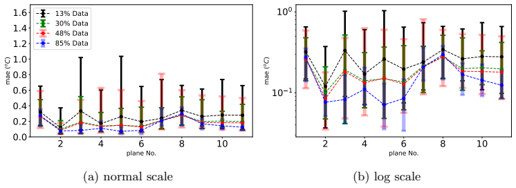
- [§5.3, Fig. 19] The authors state that "with the 48% data, the ANNGPOD method has shown poor performance than the 13% and 30% training data at most of the planes" for both 5 and 26 sensors. This non-monotonic behavior is difficult to reconcile with the abstract's claim of a "stable" method and with the introduction's claim of accurate prediction "irrespective of the number or placement of sensor points." At minimum, the robustness claim must be qualified; ideally, an explanation of why a larger training set degrades performance should be provided.
minor comments (6)
- [Table 2 and §5.4] The training proportion is given as 13% and 98% in the text but as 11% in the table caption and in the concluding remarks; please harmonize.
- [Eq. (17)] The dimension of C is stated as R^{N_r^T × N_dof}; it should be R^{N_r^T × M}.
- [Algorithm 1] Line 8 should explicitly include λ1 and λ2; as written it also omits the subscript on the GPOD loss.
- [§3.2 / §5.3] The POD-ANN method of Section 3.2 is never evaluated alone. A POD-ANN-only result would help isolate the contribution of the GPOD loss term in ANNGPOD.
- [§5.5] The advertised 'speed-up of 5e3' for ANNGPOD is per query, because the network is retrained for each new parameter value. This should be stated in the abstract/conclusions where the speed-up is advertised.
- [Throughout] There are several typos, e.g., 'Form Fig. 16b' (should be 'From'), 'M AEis' (missing space), and the abstract's '1 ( oC)'.
Circularity Check
Validation leakage into the POD basis: SVD is built from all 88 snapshots, so leave-one-out targets lie in the representation space, and ANNGPOD's sensor-loss validation includes its own input sensors.
-
fitted input called prediction
[Section 5.1 (POD-RBF basis construction); implicitly Sections 5.2-5.4]
"Singular Value Decomposition (SVD) is first applied to the dataset containing 88 parametric locations to compute the POD modes. ... Now, to employ POD-RBF ROM, We aim to reconstruct the temperature field corresponding to a particular parameter value while the rest 87 parametric points are considered to be training points ... The parameter values outside the training datasets are considered as the validation points."
In Eq. (14) all 88 configurations form the snapshot matrix, and Eq. (15) builds the POD basis by SVD on this matrix. A validation point is one of the 88 columns, so its full temperature field lies in the POD subspace up to truncation. Sections 5.2-5.3 then use this same basis in the GPOD least-squares solve (Eqs. (28)-(29)) and in the ANNGPOD sensor loss (Eqs. (31)-(32)). For a target that is in the basis and sensors that make Phi_R full column rank, the sparse data determine the target's own modal coefficients, so the 'prediction' is a reconstruction of a training snapshot. The text never states that a fresh, training-only SVD is computed for each leave-one-out split; as written, the claimed 1-degree sparse-data accuracy measures basis representability, not generalization to an unseen par
-
fitted input called prediction
[Section 5.4, ANNGPOD with Experimental Sensor Data]
"Out of 26 experimental sensors data available as shown in Fig. 3, we have considered only the middle sensors’ datasets i.e., 1.3, 2.3, 3.3, tp1 and cr3 as an input in ANNGPOD method. The temperature prediction is validated at 26 sensor locations where the experimental dataset is available."
The five middle sensors (1.3, 2.3, 3.3, tp1, cr3) are fed into ANNGPOD as inputs, and L_GPOD in Eq. (31) explicitly drives the reconstructed field to match the temperature at exactly those locations. Table 2 then reports 'ROM vs Exp' error averaged over all 26 sensor locations, including the five input sensors. Those five terms are being fitted, not predicted; the remaining 21 sensors are independent, but the reported MAE is not a purely predictive error.
full rationale
Score 7 rather than 8 because the methods still have independent content: POD-RBF's RBF coefficient interpolation and the ANN architecture do not directly use the validation full field, and the FOM-versus-experiment validation in Sec. 4.1 is genuine evidence for the CFD model. However, the central sparse-data accuracy claim in the abstract is not established as a prediction. The basis construction quoted in Sec. 5.1 includes all 88 configurations, and no text states that a training-only SVD is recomputed for the leave-one-out tests. Under Eq. (15), each validation snapshot is in the POD subspace to truncation, so GPOD's least-squares solve and ANNGPOD's GPOD loss can recover the target's own coefficients from sparse sensor data; this is fitted input renamed as prediction. The experimental-sensor validation in Sec. 5.4 additionally validates at the same five sensor locations used as input. The paper's self-citations to prior ROM work are not load-bearing, and no uniqueness theorem or imported ansatz is used. The computational speed-up claim is a runtime measurement and is not circular.
Assumptions & free parameters
free parameters (4)
- Loss weights lambda_1 and lambda_2 in Eq. 32 =
not reported
- ANN architecture and training hyperparameters =
2 hidden layers (200, 64), ReLU/Tanh activations, learning rate 0.01, decay 0.75 per 1000 steps, 20,000 epochs, seed uns
- POD truncation threshold =
99.7% cumulative energy, corresponding to 25 modes for the full dataset
- Gaussian RBF width parameter =
not reported
assumptions (5)
- ad hoc to paper All 88 simulated configurations can be used to build the POD basis while later serving as validation cases.
- domain assumption Steady RANS with k-omega SST, S2S radiation, and MRF fan modeling captures the refrigerator thermal behavior accurately enough.
- domain assumption Sparse sensor temperatures used at validation points are noise-free and mutually consistent with the high-fidelity field being reconstructed.
- domain assumption ANN training with MSE loss and backpropagation converges to a stable minimum that generalizes across the parameter space.
- ad hoc to paper The chosen training subset percentages (13%, 30%, 48%, 85%) are representative of the parameter space.
Cite this review
Pith. "Pith review of A Deep-Learning Enhanced Gappy Proper Orthogonal Decomposition Method for Conjugate Heat Transfer Problem." pith.science (2026). https://pith.science/paper/472D2NDM
@misc{pith2026250820633,
  author       = {Pith},
  title        = {Pith review of: A Deep-Learning Enhanced Gappy Proper Orthogonal Decomposition Method for Conjugate Heat Transfer Problem},
  year         = {2026},
  howpublished = {\url{https://pith.science/paper/472D2NDM}},
  note         = {Machine review of arXiv:2508.20633}
}
read the original abstract
The current study aims to develop a non-intrusive Reduced Order Model (ROM) to reconstruct the full temperature field for a large-scale industrial application based on both numerical and experimental datasets. The proposed approach is validated against a domestic refrigerator. At the full order level, air circulation and heat transfer in fluid and between fluid and surrounding solids in the fridge were numerically studied using the Conjugated Heat Transfer (CHT) method to explore both the natural and forced convection-based fridge model followed by a parametric study-based on the ambient temperature, fridge fan velocity, and evaporator temperature. The main novelty of the current work is the introduction of a stable Artificial Neural Network (ANN) enhanced Gappy Proper Orthogonal Decomposition (GPOD) method which shows better performance than the conventional GPOD approach in such large-scale industrial applications. The full-order model is validated with the experimental results and the prediction accuracy of the surrogate model associated with different reduced-order approaches is compared with the benchmark numerical results or high-fidelity results. In our current work, we show that a prediction error of one degree centigrade and computational speed-up of 5000 is achieved even at a very sparse training dataset using the proposed deep-learning enhanced GPOD approach.
Figures


Figures from the paper (17 more)




Reference graph
Works this paper leans on
-
[1]
Multi-physics simulation of an insect with flapping wings
Kabir Bakhshaei, Hoomaan MoradiMaryamnegari, Sadjad SalavatiDezfouli, Abdol Majid Khoshnood, and Mani Fathali. Multi-physics simulation of an insect with flapping wings. Proceedings of the Institution of Mechanical Engineers, Part G: Journal of Aerospace Engi- neering, 235(10):1318–1339, 2021
work page 2021
-
[2]
Optimized Bayesian Framework for Inverse Heat Transfer Problems Using Reduced Order Methods
Kabir Bakhshaei, Umberto Emil Morelli, Giovanni Stabile, and Gianluigi Rozza. Optimized bayesian framework for inverse heat transfer problems using reduced order methods. arXiv preprint arXiv:2402.19381, 2024
work page Pith review arXiv 2024
-
[3]
Stochastic Parameter Prediction in Cardiovascular Problems
Kabir Bakhshaei, Sajad Salavatidezfouli, Giovanni Stabile, and Gianluigi Rozza. Stochastic parameter prediction in cardiovascular problems. arXiv preprint arXiv:2411.18089 , 2024
work page Pith review arXiv 2024
-
[4]
C. Balaji and S.P. Venkateshan. Correlations for free convection and surface radiation in a square cavity. International Journal of Heat and Fluid Flow , 15(3):249–251, 1994
work page 1994
-
[5]
C. Balzotti, P. Siena, M. Girfoglio, A. Quaini, and G. Rozza. A data-driven Reduced Order Method for parametric optimal blood flow control: application to coronary bypass graft. Communications in Optimization Theory , 26:1–19, 2022
work page 2022
- [6]
-
[7]
R. Ben-Mansour, A. Abuelyamen, and Esmail M.A. Mokheimer. CFD analysis of radiation impact on stirling engine performance. Energy conversion and management , 152:354–365, 2017
work page 2017
-
[8]
M. D. Buhmann. Radial basis functions. Acta numerica, 9:1–38, 2000
work page 2000
Show all 58 references
-
[9]
Bui-Thanh, M
T. Bui-Thanh, M. Damodaran, and K. Willcox. Aerodynamic data reconstruction and inverse design using proper orthogonal decomposition. AIAA journal , 42(8):1505–1516, 2004
2004
-
[10]
P. J. Burns and D. V. Pryor. Surface radiative transport at large scale via monte carlo. Annual Review of Heat Transfer, 9, 1998
1998
-
[11]
B¨ uschgens, C
D. B¨ uschgens, C. Schubert, and H. Pfeifer. Radiation modelling of arbitrary two-dimensional surfaces using the surface-to-surface approach extended with a blocking algorithm. Heat and Mass Transfer, 58(9):1637–1648, 2022
2022
-
[12]
Reduced-order residential home modeling for model predictive control
Wesley J Cole, Kody M Powell, Elaine T Hale, and Thomas F Edgar. Reduced-order residential home modeling for model predictive control. Energy and Buildings , 74:69–77, 2014
2014
-
[13]
N. Demo, M. Tezzele, G. Gustin, G. Lavini, and G. Rozza. Shape optimization by means of proper orthogonal decomposition and dynamic mode decomposition. Technology and Science for the Ships of the Future: Proceedings of NA V 2018: 19th International Conference on Ship & Maritim...
2018
-
[14]
N. Demo, M. Tezzele, A. Mola, and G. Rozza. A complete data-driven framework for the efficient solution of parametric shape design and optimisation in naval engineering problems. arXiv preprint arXiv:1905.05982 , 2019
1905 arXiv
-
[15]
Shape optimization by means of proper orthogonal decomposition and dynamic mode decomposition
Nicola Demo, Marco Tezzele, Gianluca Gustin, Gianpiero Lavini, and Gianluigi Rozza. Shape optimization by means of proper orthogonal decomposition and dynamic mode decomposition. In Technology and Science for the Ships of the Future , pages 212–219. IOS Press, 2018
2018
-
[16]
An efficient shape parametri- sation by free-form deformation enhanced by active subspace for hull hydrodynamic ship de- sign problems in open source environment
Nicola Demo, Marco Tezzele, Andrea Mola, and Gianluigi Rozza. An efficient shape parametri- sation by free-form deformation enhanced by active subspace for hull hydrodynamic ship de- sign problems in open source environment. arXiv preprint arXiv:1801.06369 , 2018
2018 arXiv
-
[17]
Everson and L
R. Everson and L. Sirovich. Karhunen–loeve procedure for gappy data. JOSA A, 12(8):1657– 1664, 1995. 25
1995
-
[18]
T. L. Fine. Feedforward neural network methodology . Springer Science & Business Media, 1999
1999
-
[19]
Frank, W
A. Frank, W. Heidemann, and K. Spindler. Modeling of the surface-to-surface radiation exchange using a monte carlo method. In Journal of Physics: Conference Series , volume 745, page 032143. IOP Publishing, 2016
2016
-
[20]
Girfoglio, F
M. Girfoglio, F. Ballarin, G. Infantino, F. Nicol´ o, A. Montalto, G. Rozza, R. Scrofani, M. Comisso, and F. Musumeci. Non-intrusive podi-rom for patient-specific aortic blood flow in presence of a lvad device. Medical Engineering & Physics, 107:103849, 2022
2022
-
[21]
D. M. Godino, S. F. Corzo, and D. E. Ramajo. CFD simulation of conjugated heat transfer with full boiling in openfoam (r). Applied Thermal Engineering , 213:118627, 2022
2022
-
[22]
Gunes, S
H. Gunes, S. Sirisup, and G. Em. Karniadakis. Gappy data: To krig or not to krig? Journal of Computational Physics , 212(1):358–382, 2006
2006
-
[23]
A comparison of data-driven reduced order models for the simulation of mesoscale atmospheric flow
Arash Hajisharifi, Michele Girfoglio, Annalisa Quaini, and Gianluigi Rozza. A comparison of data-driven reduced order models for the simulation of mesoscale atmospheric flow. Finite Elements in Analysis and Design , 228:104050, 2024
2024
-
[24]
Combining ex- tended convolutional autoencoders and reservoir computing for accurate reduced-order pre- dictions of atmospheric flows
Arash Hajisharifi, Michele Girfoglio, Annalisa Quaini, and Gianluigi Rozza. Combining ex- tended convolutional autoencoders and reservoir computing for accurate reduced-order pre- dictions of atmospheric flows. arXiv preprint arXiv:2504.01097 , 2025
2025 arXiv
-
[25]
An lstm-enhanced surrogate model to simulate the dynamics of particle-laden fluid systems
Arash Hajisharifi, Rahul Halder, Michele Girfoglio, Andrea Beccari, Domenico Bonanni, and Gianluigi Rozza. An lstm-enhanced surrogate model to simulate the dynamics of particle-laden fluid systems. Computers & Fluids , 280:106361, 2024
2024
-
[26]
A non-intrusive data-driven reduced order model for parametrized cfd- dem numerical simulations
Arash Hajisharifi, Francesco Romano, Michele Girfoglio, Andrea Beccari, Domenico Bonanni, and Gianluigi Rozza. A non-intrusive data-driven reduced order model for parametrized cfd- dem numerical simulations. Journal of Computational Physics , 491:112355, 2023
2023
-
[27]
F. P. Incropera, D. P. DeWitt, Lavine Bergman, T. L., A. S., et al. Fundamentals of heat and mass transfer, volume 6. Wiley New York, 1996
1996
-
[28]
Kaplan, M
A. Kaplan, M. A. Cane, Y. Kushnir, A. C. Clement, M. B. Blumenthal, and B. Rajagopalan. Analyses of global sea surface temperature 1856–1991. Journal of Geophysical Research: Oceans, 103(C9):18567–18589, 1998
1991
-
[29]
Kim and J
D. Kim and J. Kim. Simulation of a conjugate heat transfer using a precice coupling library. In Transactions of the Korean nuclear society virtual spring meeting, July 9 , volume 10, page 2020, 2020
2020
-
[30]
Laguerre, S
O. Laguerre, S. B. Amara, J. Moureh, and D. Flick. Numerical simulation of air flow and heat transfer in domestic refrigerators. Journal of food engineering , 81(1):144–156, 2007
2007
-
[31]
Laguerre and D
O. Laguerre and D. Flick. Heat transfer by natural convection in domestic refrigerators. Journal of food engineering , 62(1):79–88, 2004
2004
-
[32]
Lahaye, P
D. Lahaye, P. Nakate, K. Vuik, F. Jureti´ c, and M. Talice. Modeling conjugate heat transfer in an anode baking furnace using openfoam. Fluids, 7(4):124, 2022
2022
-
[33]
Laitinen, K
A. Laitinen, K. Saari, K. Kukko, P. Peltonen, E. Laurila, J. Partanen, and V. Vuorinen. A computational fluid dynamics study by conjugate heat transfer in openfoam: A liquid cooling concept for high power electronics. International Journal of Heat and Fluid Flow , 85:108654, 2020
2020
-
[34]
N. C. Markatos and K.A. Pericleous. Laminar and turbulent natural convection in an enclosed cavity. International journal of heat and mass transfer , 27(5):755–772, 1984
1984
-
[35]
Mazumder
S. Mazumder. Application of a variance reduction technique to surface-to-surface monte carlo radiation exchange calculations. International Journal of Heat and Mass Transfer , 131:424– 431, 2019. 26
2019
-
[36]
F. R. Menter. Two-equation eddy-viscosity turbulence models for engineering applications. AIAA journal , 32(8):1598–1605, 1994
1994
-
[37]
N. E. Murray and L. S. Ukeiley. An application of gappy pod: For subsonic cavity flow piv data. Experiments in Fluids , 42:79–91, 2007
2007
-
[38]
Nekkanti and O
A. Nekkanti and O. T. Schmidt. Gappy spectral proper orthogonal decomposition. Journal of Computational Physics , 478:111950, 2023
2023
-
[39]
A Oliver and R
M. A Oliver and R. Webster. Kriging: a method of interpolation for geographical information systems. International Journal of Geographical Information System , 4(3):313–332, 1990
1990
-
[40]
S. V. Patankar and D. B. Spalding. A calculation procedure for heat, mass and momentum transfer in three-dimensional parabolic flows. In Numerical prediction of flow, heat transfer, turbulence and combustion , pages 54–73. Elsevier, 1983
1983
-
[41]
W. Peng, G. Li, J. Geng, and W. Yan. A strategy for the partition of mrf zones in axial fan simulation. International Journal of Ventilation , 18(1):64–78, 2019
2019
-
[42]
R. W. Reynolds and T. M. Smith. Improved global sea surface temperature analyses using optimum interpolation. Journal of climate , 7(6):929–948, 1994
1994
-
[43]
Reduced-order models for aerodynamic appli- cations, loads and mdo
Matteo Ripepi, Mark Johannes Verveld, NW Karcher, Thomas Franz, Mohammad Abu- Zurayk, Stefan G¨ ortz, and Thiemo M Kier. Reduced-order models for aerodynamic appli- cations, loads and mdo. CEAS Aeronautical Journal, 9(1):171–193, 2018
2018
-
[44]
Rojas and R
R. Rojas and R. Rojas. The backpropagation algorithm. Neural networks: a systematic introduction, pages 149–182, 1996
1996
-
[45]
D. E. Rumelhart, G. E. Hinton, and R. J. Williams. Learning representations by back- propagating errors. nature, 323(6088):533–536, 1986
1986
-
[46]
C. L. Rumsey. Compressibility considerations for kw turbulence models in hypersonic boundary-layer applications. Journal of Spacecraft and Rockets , 47(1):11–20, 2010
2010
-
[47]
Modal analysis of the wake shed behind a horizontal axis wind turbine with flexible blades
Sajad Salavatidezfouli, Armin Sheidani, Kabir Bakhshaei, Ali Safari, Arash Hajisharifi, Gio- vanni Stabile, and Gianluigi Rozza. Modal analysis of the wake shed behind a horizontal axis wind turbine with flexible blades. Journal of Applied and Computational Mechanics , 11(3):8...
2025
-
[48]
Sekar, Q
V. Sekar, Q. Jiang, C. Shu, and Boo C. Khoo. Fast flow field prediction over airfoils using deep learning approach. Physics of Fluids , 31(5), 2019
2019
-
[49]
Sharma, Simone S., and A
S. Sharma, Simone S., and A. Athaiya. Activation functions in neural networks. Towards Data Sci , 6(12):310–316, 2017
2017
-
[50]
T. M. Smith, R. W. Reynolds, R. E. Livezey, and D. C. Stokes. Reconstruction of historical sea surface temperatures using empirical orthogonal functions. Journal of Climate , 9(6):1403– 1420, 1996
1996
-
[51]
S¨ oylemez, E
E. S¨ oylemez, E. Alpman, A. Onat, and S. Hartomacıo˘ glu. Cfd analysis for predicting cooling time of a domestic refrigerator with thermoelectric cooling system. International Journal of Refrigeration, 123:138–149, 2021
2021
-
[52]
G Weller, G
H. G Weller, G. Tabor, H. Jasak, and C. Fureby. A tensorial approach to computational continuum mechanics using object-oriented techniques. Computers in physics , 12(6):620–631, 1998
1998
-
[53]
D. C. Wilcox. Formulation of the kw turbulence model revisited. AIAA journal, 46(11):2823– 2838, 2008
2008
-
[54]
K. Willcox. Unsteady flow sensing and estimation via the gappy proper orthogonal decompo- sition. Computers & fluids , 35(2):208–226, 2006. 27
2006
-
[55]
A co- simulation method of refrigerator system and temperature field
Shijie Xu, Min Wang, Lili Han, Shoujie Zhang, Jianlin Yu, and Suxin Qian. A co- simulation method of refrigerator system and temperature field. Applied Thermal Engineering, 235:121412, 2023
2023
-
[56]
Yakhot, T
A. Yakhot, T. Anor, and G. E.m. Karniadakis. A reconstruction method for gappy and noisy arterial flow data. IEEE transactions on medical imaging , 26(12):1681–1697, 2007
2007
-
[57]
Z Yousif, L
M. Z Yousif, L. Yu, S. Hoyas, R. Vinuesa, and H. Lim. A deep-learning approach for recon- structing 3d turbulent flows from 2d observation data. Scientific Reports, 13(1):2529, 2023
2023
-
[58]
Zhang and Y
C. Zhang and Y. Lian. Conjugate heat transfer analysis using a simplified household refriger- ator model. International journal of refrigeration , 45:210–222, 2014. 28
2014
Reviewed August 5, 2026 · model on record in the stance chip above.
Discussion (0). Continue with ORCID to comment.