REVIEW 3 major objections 5 minor 1 cited by
Prediction of EDS Maps from 4DSTEM Diffraction Patterns Using Convolutional Neural Networks
T0 review · 3 major / 5 minor · reviewed 2026-08-05 · deepseek-v4-flash
Pith's one-line read The paper reports that a convolutional neural network can infer elemental composition maps directly from 4D-STEM diffraction patterns, with strongest accuracy for high-contrast elements such as oxygen and tellurium.
desk verdict Plausible proof-of-concept for direct 4D-STEM-to-EDS mapping, but blurred targets and repeated scans of one sample leave the accuracy claim untested against a trivial spatial-prior baseline. read the letter →
The pith
A machine-rendered reading of the paper's core claim, the machinery that carries it, and where it could break.
The reading
What carries the argument
The engine is a convolutional neural network—a layered image-processing model that learns spatial features—mapping each 256×256 diffraction pattern to five elemental concentration maps. The training targets are EDS maps smoothed with a Gaussian blur (kernel width 7), because raw EDS maps are grainy. The improved pipeline adds a linear calibration y = αyCNN + β after the network and uses HAADF images as an auxiliary output, which forces the network to learn structural features shared by both signals. Cross-correlation matrices of the predicted element maps are used to check that inter-element relationships survive prediction.
What would settle it
Retrain the same CNN using raw, unblurred EDS maps as training targets and test on the same held-out files. If the Pearson correlations for oxygen and tellurium collapse toward zero, the blur is doing most of the work; if they persist, the diffraction-to-chemistry mapping is real.
Extended reading notes
Core claim
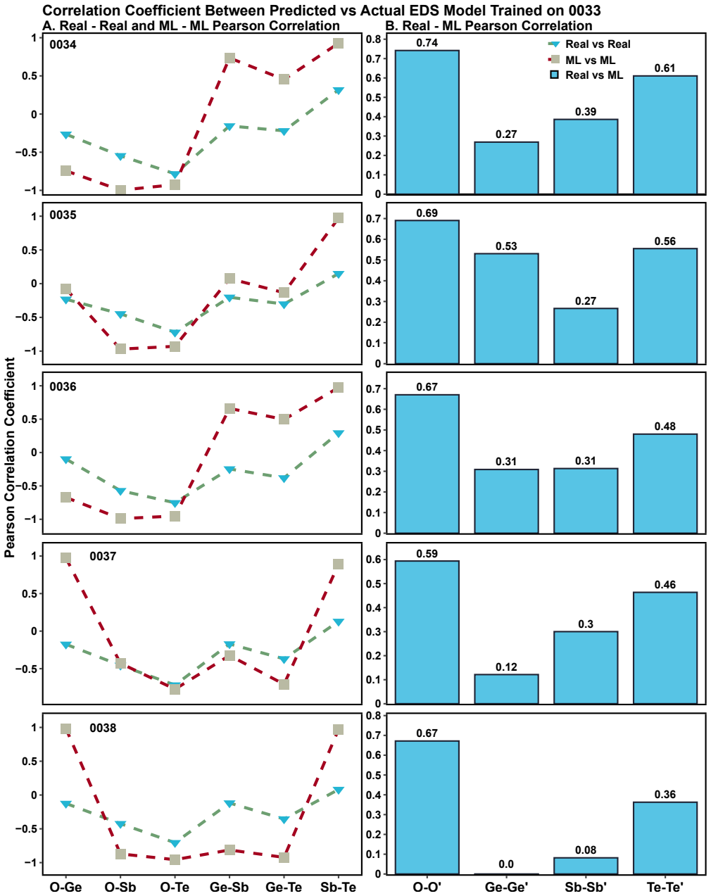
The central claim is that 4D-STEM diffraction patterns carry enough structural information to infer elemental composition, and that a CNN can learn that mapping from paired data without any physics-based model of scattering. The paper reports that under an 80/20 split within one scan file, correlations between predicted and measured compositions reach 0.981, 0.950, 0.933, 0.959, and 0.986 for O, Si, Ge, Sb, and Te. In the harder cross-file extrapolation test (train on one file, test on five others), average correlations fall to 0.68 (O), 0.017 (Si), 0.24 (Ge), 0.26 (Sb), and 0.47 (Te), and interpolation between endpoint files gives a slight improvement for Ge, Sb, and Te. Visual inspection s
Load-bearing premise
The agreement is measured against Gaussian-blurred EDS maps, so the reported accuracy could partly reflect the smoothness of both the target and the network output rather than a true chemical signal.
Editorial extensions
If this is right
- EDS acquisition time and electron dose could be reduced because composition maps would be derived from the 4D-STEM data already being collected.
- The same architecture should transfer to other multi-element samples, with accuracy expected to scale with element concentration and diffraction contrast.
- Including HAADF as an auxiliary training output improves chemical prediction, suggesting multimodal training is a general route to quantitative accuracy.
- Training on boundary files and predicting intermediate ones works, so the approach could track slow compositional drift in a series of scans.
Reading between the lines
- Because the EDS targets were Gaussian-blurred, the reported correlations likely overstate sensitivity to fine-scale composition; a raw-target test would clarify this. (Editorial inference.)
- The architecture should be retested on multiple instruments and sample geometries to see whether the learned diffraction-to-chemistry mapping is transferable beyond this Ge-Sb-Te dataset. (Editorial inference.)
- The same structure-to-chemistry regression could be applied to predict other spectral maps, such as EELS, from diffraction alone. (Editorial inference.)
- The model's smoothing bias suggests a practical use as an anomaly detector: regions where predicted and measured maps disagree sharply may mark chemistry that departs from the dominant structure-chemistry correlation. (Editorial inference.)
Editorial analysis
A structured set of objections, weighed in public.
Referee Report
Summary. The paper proposes a convolutional neural network (CNN) to predict elemental composition maps from 4D-STEM diffraction patterns of a Ge-Sb-Te phase-change material. The authors first train on an 80/20 random split of one file (0033) and report high Pearson correlations (0.93-0.99) against Gaussian-blurred EDS maps. They then test two generalization strategies: extrapolation (train on file 0033, test on files 0034-0038) and interpolation (train on files 0033 and 0038, test on 0034-0037). In both cases, mean correlations are moderate for O (≈0.68) and Te (≈0.47-0.50), weak for Ge and Sb, and near zero for Si. A final section describes a hybrid model that adds HAADF output and linear calibration, reporting reduced MAE on one file. The central claim is that the CNN 'accurately infers elemental compositions' from diffraction patterns, enabling faster and less damaging chemical mapping.
Significance. If the central claim were established, the work would be a useful proof-of-concept for reducing EDS acquisition time in 4D-STEM, and the pairing of paired experimental diffraction and EDS data with explicit cross-file evaluation is a strength. The manuscript also includes code snippets for preprocessing and model architecture, which aids reproducibility. However, the current evidence does not yet support the claim: the evaluation is performed against Gaussian-blurred targets, and no baseline predictor is compared, so the reported correlations may reflect spatial autocorrelation and repeated scans of a single specimen rather than diffraction-driven inference. The cross-file tests are a step beyond purely circular evaluation, but they remain within one sample. With additional baseline comparisons and a more cautious interpretation, the result could become convincing.
major comments (3)
- [Training on One File, Predicting on Others (pp. 3-5), Fig. 2] No trivial baseline is reported. All files 0033-0038 are repeated scans of the same Ge-Sb-Te specimen, and the EDS targets are Gaussian blurred with a 7×7 kernel (Code 2). The CNN output is also strongly smoothed by five max-pooling layers and an MAE objective (Code 3). Under these conditions, a predictor that simply outputs the blurred mean O or Te map from the training file would share large-scale spatial structure with the test maps and could produce substantial Pearson correlations. Without comparing to such a baseline, or to a model trained on shuffled diffraction patterns, the correlations in Fig. 2A do not establish that the predictions are driven by diffraction-pattern content. This is load-bearing for the abstract's 'accurately infers elemental compositions.'
- [Materials and Methods, Data Preparation / Code 2 and Fig. 9] The evaluation treats Gaussian-blurred EDS maps as ground truth. Blurring removes high-frequency noise and increases spatial autocorrelation, so correlation between two smooth maps (prediction and blurred target) is inflated relative to correlation with raw, grainy EDS. The reported MAE values (e.g., 0.035 for O in the extrapolation test) are errors against blurred targets, not against the measured EDS signal. The authors should either validate against unblurred EDS maps, report how the blur affects the metrics, or explicitly reframe the claim as predicting a smoothed version of EDS maps rather than 'elemental compositions' without qualification.
- [First Approach and Data Preparation (pp. 4-5, 10-11)] The manuscript claims a 'generalized machine learning model' and features 'independent of sample-specific variations,' but only one specimen is used, and the six files are consecutive scans of the same region. The 'unseen' files share sample geometry, drift, and thickness variations, so the extrapolation/interpolation tests assess stability across repeated scans, not transfer to a new sample or material. The conclusions should be scoped accordingly, and the term 'generalization' should be defined more carefully to avoid implying cross-sample generalizability that the data cannot support.
minor comments (5)
- [Choosing Machine Learning Model (p. 12)] The sentence 'After the preprocessing in section ' has an empty cross-reference; a specific section number is needed.
- [Code 3 and Improving the Accuracy of the Model (p. 9)] Code 3 shows a final softmax layer with MAE loss, while the 'Improving the Accuracy' section states the output activation 'was changed to Relu.' The manuscript should specify which model variant was used for each reported result and whether the softmax/MAE combination was retained in the hybrid model.
- [Fig. 5B] The y-axis label contains a typo: 'Mean Absolute Errur' should be 'Mean Absolute Error.'
- [Data Preparation (p. 11)] The Gaussian blur is described as a 'channel width of 7'; in OpenCV, this is a kernel size of 7×7, which is clearer and matches Code 2.
- [Figure 1B] The x-axis label 'Samples' is ambiguous; these appear to be individual pixels or scan positions, not independent samples. Please clarify the unit.
Circularity Check
Core CNN-vs-EDS prediction is not circular, but the reported post-hoc linear-calibration improvement is a fitted value unless evaluated on a held-out split.
-
fitted input called prediction
[Improving the Accuracy of the Model (Eq. 1 and Figure 8A)]
"A simple linear calibration model is defined as, y ≡ αyCNN + β (1) Where, α and β are the regression coefficients determined after the training of linear regressor. ... After training the CNN ... we observed a substantial improvement in predictive performance. The mean absolute error (MAE) decreased significantly, reaching values as low as 0.0097."
The calibration coefficients α and β are fit to map the CNN output yCNN to the ground-truth EDS value y. The paper then reports the resulting MAE improvement without stating that this evaluation was performed on a held-out split that was not used to fit α and β. If the MAE is computed on the same data used to determine α and β, the improvement is a least-squares artifact: the calibrated output is the fitted value itself, not a prediction. The equation's use of the identity symbol '≡' makes the fitted relation explicit, and no cross-validation or separate calibration set is described. Thus the 'substantial improvement' in predictive performance is statistically forced by construction.
full rationale
The paper's central derivation is a standard supervised regression from 4D-STEM diffraction patterns to EDS composition maps, with file-level held-out splits (training on 0033 and testing on 0034–0038, or training on 0033/0038 and testing on 0034–0037). That design is not circular in the definitional sense: the model is not given EDS values at test time, and the reported correlations are genuine out-of-sample predictions with respect to file separation. No load-bearing self-citation chain or imported uniqueness theorem is present. The main circularity concern is confined to the 'Improving Accuracy' section, where a linear calibration y ≡ αyCNN + β is fit to the ground-truth y and the resulting MAE is reported without an explicit held-out calibration split; that specific reported improvement reduces to a fitted value. Separate methodological issues—Gaussian-blurred EDS targets, repeated scans of a single specimen, and the absence of a trivial baseline—could confound the magnitude of the reported correlations, but they are not definitional circularity because the CNN still receives diffraction input and the test files are not used in training. Accordingly, the central claim retains independent content, and the score reflects one secondary circular step rather than a fully circular derivation.
Assumptions & free parameters
free parameters (7)
- CNN trainable weights =
not reported
- Learning rate (Adam) =
0.0001
- Batch size =
64
- Gaussian blur kernel size for EDS targets =
7x7, sigma 0
- Crop range =
[20*45:90*45]
- EarlyStopping patience =
5
- Linear calibration coefficients alpha, beta =
not reported
assumptions (4)
- domain assumption EDS composition maps are correlated with 4D-STEM diffraction patterns in this sample system.
- domain assumption Files 0033-0038 are sufficiently independent to serve as external test sets for generalization.
- domain assumption Gaussian-blurred EDS maps are an appropriate ground truth for training and evaluation.
- ad hoc to paper A softmax output layer with MAE loss is appropriate for predicting elemental composition maps.
Cite this review
Pith. "Pith review of Prediction of EDS Maps from 4DSTEM Diffraction Patterns Using Convolutional Neural Networks." pith.science (2026). https://pith.science/paper/YXQKIWCH
@misc{pith2026250820657,
  author       = {Pith},
  title        = {Pith review of: Prediction of EDS Maps from 4DSTEM Diffraction Patterns Using Convolutional Neural Networks},
  year         = {2026},
  howpublished = {\url{https://pith.science/paper/YXQKIWCH}},
  note         = {Machine review of arXiv:2508.20657}
}
read the original abstract
Understanding the relationship between atomic structure (order) and chemical composition (chemistry) is critical for advancing materials science, yet traditional spectroscopic techniques can be slow and damaging to sensitive samples. Four-dimensional scanning transmission electron microscopy (4D-STEM) captures detailed diffraction patterns across scanned regions, providing rich structural information, while energy dispersive X-ray spectroscopy (EDS) offers complementary chemical data. In this work, we develop a machine learning framework that predicts EDS spectra directly from 4D-STEM diffraction patterns, reducing beam exposure and acquisition time. A convolutional neural network (CNN) accurately infers elemental compositions, particularly for elements with strong diffraction contrast or higher concentrations, such as Oxygen and Tellurium. Both extrapolation and interpolation strategies demonstrate consistent performance, with improved predictions when additional structural context is available. Visual and cross-correlation analyses confirm the model's ability to capture global and local compositional trends. This approach establishes a data-driven pathway to non-destructive, high-throughput materials characterization.
Figures


Figures from the paper (7 more)


Forward citations
Cited by 1 Pith paper
-
Protocol for Clustering 4DSTEM Data for Phase Differentiation in Glasses
Clustering 4D-STEM diffraction data from Ge-Sb-Te with PCA, UMAP, and k-means yields four spatial clusters with distinct elemental intensity signatures.
Reference graph
Works this paper leans on
-
[1]
Savitzky, B. H. et al. py4DSTEM: Open source software for 4D-STEM data analysis. Microsc. Microanal. 25, 124–125, DOI: 10.1017/S1431927619001351 (2019). https://academic.oup.com/mam/article-pdf/25/S2/124/48323359/mam0124. pdf
-
[2]
Savitzky, B. H. et al. py4DSTEM: A software package for four-dimensional scanning transmission electron microscopy data analysis. Microsc. Microanal. 27, 712–743, DOI: 10.1017/S1431927621000477 (2021). 13/14
-
[3]
Chapter 4.4 - energy-dispersive x-ray spectroscopy (EDS)
Hodoroaba, V .-D. Chapter 4.4 - energy-dispersive x-ray spectroscopy (EDS). In Hodoroaba, V .-D., Unger, W. E. & Shard, A. G. (eds.) Characterization of Nanoparticles , Micro and Nano Technologies, 397–417, DOI: 10.1016/ B978-0-12-814182-3.00021-3 (Elsevier, 2020)
work page 2020
-
[4]
Schmied, M. & Poelt, P. Particle Analysis by SEM/EDXS and Specimen Damage. Microchimica Acta 139, 171–177, DOI: 10.1007/s006040200057 (2002)
-
[5]
Wei, J. et al. Machine learning in materials science. InfoMat 1, 338–358, DOI: 10.1002/inf2.12028 (2019). https: //onlinelibrary.wiley.com/doi/pdf/10.1002/inf2.12028
-
[6]
Zhang, C., Feng, J., DaCosta, L. R. & V oyles, P. M. Atomic resolution convergent beam electron diffraction analysis using convolutional neural networks. Ultramicroscopy 210, 112921 (2020)
work page 2020
-
[7]
Sadri, A. et al. Unsupervised deep denoising for four-dimensional scanning transmission electron microscopy. NPJ Comput. Mater. 10, 243 (2024)
2024
-
[8]
Machine Learning (Springer nature, 2021)
Zhou, Z.-H. Machine Learning (Springer nature, 2021)
work page 2021
Show all 12 references
-
[9]
Wei, J. et al. Machine learning in materials science. InfoMat 1, 338–358 (2019)
2019
-
[10]
Agrawal, A. et al. Exploration of data science techniques to predict fatigue strength of steel from composition and processing parameters. Integrating materials manufacturing innovation 3, 90–108 (2014)
2014
-
[11]
Bradski, G., Kaehler, A. et al. OpenCV. Dr . Dobb’s journal software tools3 (2000)
2000
-
[12]
& Keyes, R
Wen, T. & Keyes, R. Time series anomaly detection using convolutional neural networks and transfer learning. arXiv preprint arXiv:1905.13628 (2019). 1905.13628. 14/14
1905 arXiv
Reviewed August 5, 2026 · model on record in the stance chip above.
Discussion (0). Continue with ORCID to comment.