REVIEW 3 major objections 4 minor 47 references
Antihydrogen beam intensity rises 100-fold, and the beam's velocity and binding-energy distributions are measured in enough detail to plan a ground-state hyperfine measurement.
Reviewed by Pith at T0; open to challenge. T0 means a machine referee read the full paper against a public rubric. the ladder, T0–T4 →
ASACUSA reports a 100x more intense antihydrogen beam, measures its velocity and Rydberg-state distribution, and estimates a 16% ground-state fraction useful for future hyperfine spectroscopy.
T0 review reviewed 2026-08-05 challenge →
load-bearing objection Solid direct measurements; the 16% ground-state fraction is a simulation extrapolation with a tuned cutoff, so treat the 50-hour hyperfine projection with skepticism. the 3 major comments →
Measured Properties of an Antihydrogen Beam
The pith
A machine-rendered reading of the paper's core claim, the machinery that carries it, and where it could break.
The reading
Core claim
The central claim is that the antihydrogen beam is now intense enough and well enough characterized to plan a beam-based measurement of the ground-state hyperfine splitting. The measured beam delivers 320 atoms per 15-minute run downstream of the Cusp trap, a 100-fold increase over previous antihydrogen-beam experiments. Time-of-flight and field-ionization data yield a 1D Maxwellian axial velocity distribution with a temperature near 1500 K, a binding-energy distribution concentrated at n≈20–50, a newly observed correlation between lower n and lower velocity, and a simulation-based estimate that about 16% of formed atoms are in the ground state. The authors also demonstrate that detected cou
What carries the argument
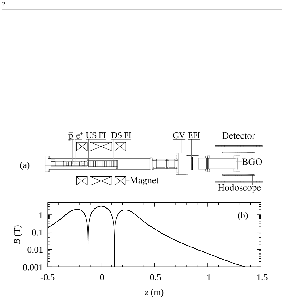
The Cusp trap's double anti-Helmholtz coils create two magnetic nulls that focus low-field-seeking atoms into a beam of fractional solid angle 2.1e-4. Two in-trap field ionizers and an external ionizer selectively ionize Rydberg atoms; the conversion from field strength to principal quantum number n follows the classical threshold range 1/(7.7 n^4) < F < 1/(2.6 n^4). Three protocols—pulsed without blocking, pulsed with blocking, and a triangle-wave ramp—turn beam intensity into time-of-flight and binding-energy distributions. A Monte Carlo formation simulation, fed by plasma temperature, density, transit time, blackbody radiation temperature, and an upper principal-quantum-number cutoff, con
Load-bearing premise
The load-bearing premise is that the simulation's prediction of a 16 percent ground-state fraction is sound, even though matching the measured data requires setting an upper principal-quantum-number cutoff near 45 and the simulation omits how the Cusp magnet's field gradients remove high-n atoms; if that omission biases the ground-state yield, the projected 50 slow ground-state atoms per run and the 50-hour spectroscopy timeline would be wrong.
What would settle it
The ground-state estimate comes from a simulation with an unmodeled loss channel, so the decisive check is a direct count of ground-state atoms. One concrete way: insert the spectroscopy apparatus in the beam and look for the hyperfine resonance signal; if the observed per-run rate of slow ground-state atoms is far from about 50, the 16% fraction is wrong. A quicker experimental check would be to add an extra magnetic-field-gradient section between trap and detector and measure whether the n=1 yield changes by more than the quoted few percent; if it does, the omission is not benign.
If this is right
- A first in-beam measurement of the antihydrogen ground-state hyperfine splitting could be feasible with about 200 15-minute runs, or roughly 50 hours, assuming about 50 slow ground-state atoms are detected per run.
- Over 30% of the beam atoms have axial velocities below 1500 m/s and are slow enough for the ASACUSA spectrometer.
- Because detected intensity scales linearly with the number of antiprotons over an order of magnitude, increasing the antiproton number toward 10^7 per run should raise the beam intensity correspondingly.
- The newly observed correlation between lower principal quantum number and lower velocity implies that ground-state atoms tend to be the slowest, which is favorable for beam spectroscopy.
- The ionizable part of the beam peaks at n ≈ 20–50, consistent with formation by three-body recombination followed by collisional deexcitation.
Where Pith is reading between the lines
- If the unmodeled loss of high-n atoms in the Cusp field gradients also removes a different fraction of low-n atoms, the simulated 16% ground-state fraction could be biased; a direct measurement of the n=1 population would settle whether the 50-hour projection is realistic.
- The n-v correlation suggests a possible lever: deliberately selecting low-n atoms by tuning the field ionizer could enrich the slow, spectroscopically useful part of the beam, at the cost of intensity.
- The linear rate scaling with antiproton number is measured over about one order of magnitude; whether it extends to 10^7 antiprotons depends on plasma-related losses that the paper defers to future work.
- Applying the same pulsed-field-ionization time-of-flight method to hydrogen should provide a calibration of the simulation's ground-state fraction under similar plasma conditions, since the atomic physics is identical.
Editorial analysis
A structured set of objections, weighed in public.
Referee Report
Summary. The paper reports a factor-of-100 increase in the antihydrogen beam intensity downstream of ASACUSA's Cusp trap, with 320 atoms detected per 15-minute run, and characterizes the beam using field ionization and time-of-flight methods. A 1D Maxwellian velocity distribution with T_m ≈ 1500 K fits the ToF data, the ionizable atoms mostly have n between 20 and 50, and a lower-n/lower-velocity correlation is inferred. A classical-trajectory Monte Carlo simulation is used to estimate that about 16% of formed atoms may be in the ground state, and this figure feeds a projection that an in-beam hyperfine measurement may be feasible in about 50 hours. The beam intensity is also shown to scale linearly with the antiproton number over one order of magnitude.
Significance. If the direct measurements stand, this is a major step for antihydrogen beam spectroscopy: the 100-fold intensity increase, the careful field-ionization calibration validated at three ionizer positions, the bootstrap uncertainties, and the open data are all concrete strengths. However, the 16% ground-state fraction is not measured but derived from a simulation whose upper cutoff n_lim is effectively tuned to match a detected n distribution that has already been filtered by unmodeled magnetic-field-gradient losses. The feasibility projection for hyperfine spectroscopy therefore rests on an extrapolation with unquantified systematic uncertainty. The paper is still well within the scope of physics.ins-det and the direct measurements are likely correct, but the ground-state fraction claim needs substantial strengthening before acceptance.
major comments (3)
- [§3, 'We compare the simulation result with Fig. 2(c)...'] The statement that the ground-state prediction 'does not depend on any free parameters' is not supported. The simulation's normalization depends on n_lim, and the text says best agreement with the measured n distribution occurs for n_lim≈45, while n_lim≈80 would be physically expected. Only n_lim = 40, 50, 60 are shown in Fig. 3. Because the probability is normalized to the sum up to n_lim, the 16±2% ground-state fraction could depend strongly on this cutoff; the sensitivity to n_lim≈80 has not been explored. Please provide this sensitivity analysis or clearly rephrase the claim as conditional on n_lim.
- [§3, 'One possible explanation is that the B gradients in the Cusp remove atoms with a large magnetic moment...'] The paper explicitly states that magnetic-field-gradient removal of high-n atoms is not included in the simulation. Yet the measured n distribution used to validate the simulation is obtained after this same loss process. Using that truncated distribution to choose n_lim and then normalizing the ground-state fraction over the truncated range risks a circular argument. A quantitative estimate of the gradient-loss bias, or at least a model bounding the effect on the 16% figure, is needed before this number can support the 50-hour spectroscopy projection.
- [§3, protocols (a) and (b), fitted T_m values] The claimed lower-n/lower-velocity correlation is based on T_m = 1510±190 K for protocol (a) and 1150±140 K for protocol (b), a difference of about 1.5σ, plus an indirect delay estimate. This is suggestive but not yet a robust observation. Since the paper later uses 'ground state atoms will also be the slowest atoms' as a premise for the 50 slow-atom-per-run projection, the correlation needs either a stronger statistical statement or explicit hedging in the conclusion.
minor comments (4)
- [Abstract and §3] The abstract says 'about 16% of the atoms may be in the ground state' but the body gives 16±2% as an averaging result over four simulation models. Please make the provisional nature consistent, and explain why the four models are averaged rather than used to define a systematic range.
- [Fig. 3] The right-hand axis label 'Binding energy (K)' is not defined in the caption. Specify the conversion from principal quantum number n to binding energy in kelvin.
- [Appendix B] The analysis uses the B=0.35 T ionization curve as a 'conservative estimate' for the in-trap FIs, although the field ranges from 0.1 to 0.35 T. State explicitly whether this choice introduces a systematic offset in the n ranges, and why it is conservative for both the intensity and the n-velocity correlation.
- [Data availability, Ref. [46]] The Zenodo link contains a long preview token and may be embargoed. Please provide a stable DOI link without private tokens.
Circularity Check
No significant circularity: the beam measurements are direct and the 16% ground-state simulation is a forward CTMC calculation validated against, not fitted to, the measured n-distribution.
full rationale
The paper's central measurements—320 atoms per run, ToF temperature ~1500 K, binding-energy distribution, and the n-velocity correlation—are direct detector observations analyzed with standard models; none are defined in terms of the conclusions. The 16% ground-state fraction is taken from a classical-trajectory Monte Carlo simulation [33] using measured plasma inputs; the simulation is not fitted to the ground-state number, and the comparison with Fig. 2(c) is a validation of the modeled n distribution, not a fit to the target quantity. The n_lim parameter is varied over 40–60 (plus a 300 K case) and the reported spread is ~2%; the paper explicitly identifies the B-gradient loss of high-n atoms as an unmodeled effect that may explain why n_lim≈45 is lower than the physically expected ~80. That is an acknowledged limitation and a correctness risk for the 50-hour projection, but not circular reasoning: the ground-state fraction is not forced by the measured data by construction. The only self-citation in the chain (Ref. [33], with coauthor overlap) supplies a published simulation, not an imported uniqueness theorem, and the present paper checks its output against independent FI measurements. The direct experimental results are self-contained and externally benchmarked, so no circularity score is warranted.
Axiom & Free-Parameter Ledger
free parameters (4)
- T_m (protocol a) =
1510 +/- 190 K
- T_m (protocol b) =
1150 +/- 140 K
- Triangle-wave time delay =
0.65 +/- 0.05 ms
- Simulation upper limit n_lim =
varied 40, 50, 60; best agreement near 45
axioms (5)
- domain assumption The antihydrogen velocity distribution along the beam axis is a 1D Maxwellian, exp[-v^2/(2 v_t^2)].
- domain assumption The classical-trajectory Monte Carlo simulation of Radics et al. (Ref. [33]) correctly describes Hbar formation from mixing plasmas and is a valid basis for the ground-state fraction estimate.
- domain assumption The positron plasma density is 1.8e8 cm^-3, calculated from known plasma and trap properties rather than measured directly in this run.
- standard math The classical field-ionization thresholds computed for H in magnetic fields up to 0.35 T correctly map FI voltages to principal quantum number ranges.
- domain assumption The 80 count/run background measured with the gate valve closed is treated as representative for all mixing runs.
Cite this review
Pith. "Pith review of Measured Properties of an Antihydrogen Beam." pith.science (2026). https://pith.science/paper/UWHADQDZ
@misc{pith2026250902583,
  author       = {Pith},
  title        = {Pith review of: Measured Properties of an Antihydrogen Beam},
  year         = {2026},
  howpublished = {\url{https://pith.science/paper/UWHADQDZ}},
  note         = {Machine review of arXiv:2509.02583}
}
abstract
We report a factor of $100$ increase in the antihydrogen beam intensity downstream of ASACUSA's Cusp trap: $320$ atoms detected per $15$-minute run. The beam contains many Rydberg atoms, which we selectively ionize to determine their velocity and binding energy. The time of flight signal is modeled using a $1\mathrm{D}$ Maxwellian velocity distribution with a temperature of $1500\,\mathrm{K}$, which is close to the measured antiproton plasma temperature. A numerical simulation reproduces the observed distribution of binding energies and suggests that about $16\%$ of the atoms may be in the ground state.
Figures


Reference graph
Works this paper leans on
-
[1]
M. Ahmadi, B.X.R. Alves, C.J. Baker, W. Bertsche, E. Butler, A. Capra, C. Carruth, C.L. Cesar, M. Charlton, S. Cohen, R. Collister, S. Eriksson, A. Evans, N. Evetts, J. Fajans,et al., Observation of the hyperfine spectrum of antihydrogen, Nature 548 (2017), pp. 66–69, Available athttps: //doi.org/10.1038/nature23446
-
[2]
S.G.Karshenboim, Precisionphysicsofsimpleatoms: Qedtests,nuclearstructureandfundamental constants, Phys. Rep. 422 (2005), pp. 1–63, Available athttps://www.sciencedirect.com/ science/article/pii/S0370157305003637
work page 2005
-
[3]
L. Nowak, C. Malbrunot, M. Simon, C. Amsler, S. Arguedas Cuendis, S. Lahs, A. Lanz, A. Nanda, M. Wiesinger, T. Wolz, and E. Widmann,Cpt and lorentz symmetry tests with hydrogen using a novel in-beam hyperfine spectroscopy method applicable to antihydrogen experiments, Phys. Lett. B858(2024),p.139012,Availableat https://doi.org/10.1016/j.physletb.2024.139012
arXiv 2024
-
[4]
E. Widmann, R. Hayano, M. Hori, and T. Yamazaki,Measurement of the hyperfine structure of antihydrogen, Nucl. Instrum. Methods Phys. Res., Sect. B 214 (2004), pp. 31–34, Available at https://www.sciencedirect.com/science/article/pii/S0168583X03019116, low En- ergy Antiproton Physics (LEAP’03)
work page 2004
-
[5]
E. Widmann, M. Diermaier, B. Juhász, C. Malbrunot, O. Massiczek, C. Sauerzopf, K. Suzuki, B. Wünschek, J. Zmeskal, S. Federmann, N. Kuroda, S. Ulmer, and Y. Yamazaki,Measurement of the hyperfine structure of antihydrogen in a beam, Hyperfine Interact. 215 (2013), pp. 1–8
work page 2013
-
[6]
G. Gabrielse, A. Speck, C.H. Storry, D. LeSage, N. Guise, D. Grzonka, W. Oelert, G. Schepers, T. Sefzick, H. Pittner, J. Walz, T.W. Hänsch, D. Comeau, and E.A. Hessels,First measurement of the velocity of slow antihydrogen atoms, Phys. Rev. Lett. 93 (2004), p. 073401, Available at https://link.aps.org/doi/10.1103/PhysRevLett.93.073401
-
[7]
G. Gabrielse, N.S. Bowden, P. Oxley, A. Speck, C.H. Storry, J.N. Tan, M. Wessels, D. Grzonka, W. Oelert, G. Schepers, T. Sefzick, J. Walz, H. Pittner, T.W. Hänsch, and E.A. Hessels,Driven productionofcoldantihydrogenandthefirstmeasureddistributionofantihydrogenstates ,Phys.Rev. Lett.89(2002),p.233401,Availableat https://link.aps.org/doi/10.1103/PhysRevLet...
-
[8]
B.Kolbinger,C.Amsler,S.A.Cuendis,H.Breuker,A.Capon,G.Costantini,P.Dupré,M.Fleck,A. Gligorova, H. Higaki, Y. Kanai, V. Kletzl, N. Kuroda, A. Lanz, M. Leali, V. Mäckel, C. Malbrunot, V.Mascagna,O.Massiczek,Y.Matsuda,D.J.Murtagh,Y.Nagata,A.Nanda,L.Nowak,B.Radics, C.Sauerzopf,M.C.Simon,M.Tajima,H.A.Torii,U.UggerhØj,S.Ulmer,L.Venturelli,A.Weiser, M. Wiesinger,...
work page 2021
-
[9]
M. Ahmadi, B.X.R. Alves, C.J. Baker, W. Bertsche, E. Butler, A. Capra, C. Carruth, C.L. Cesar, M. Charlton, S. Cohen, R. Collister, S. Eriksson, A. Evans, N. Evetts, J. Fajans, T. Friesen, M.C. Fujiwara, D.R. Gill, A. Gutierrez, J.S. Hangst, W.N. Hardy, M.E. Hayden, C.A. Isaac, A. Ishida, M.A.Johnson, S.A.Jones, S.Jonsell, L.Kurchaninov, N.Madsen, M.Mathe...
work page 2017
-
[10]
S. Maury, W. Oelert, W. Bartmann, P. Belochitskii, H. Breuker, F. Butin, C. Carli, T. Eriksson, S. Pasinelli,andG.Tranquille, Elena: theextralowenergyanti-protonfacilityatcern ,HyperfineInter- act. 229 (2014), pp. 105–115, Available athttps://doi.org/10.1007/s10751-014-1067-y
-
[11]
A. Lanz, C. Amsler, H. Breuker, M. Bumbar, S. Chesnevskaya, G. Costantini, R. Ferragut, M. Giammarchi, A. Gligorova, G. Gosta, H. Higaki, C. Killian, V. Kraxberger, N. Kuroda, M. Leali, G. Maero, C. Malbrunot, V. Mascagna, Y. Matsuda, V. Mäckel, S. Migliorati, D. Murtagh, A. Nanda, L. Nowak, F. Parnefjord Gustafsson, S. Rheinfrank, M. Romé, M. Simon, M. T...
work page internal anchor Pith review Pith/arXiv arXiv doi:10.48550/arxiv.2307.06133 2023
-
[12]
G. Gabrielse, S.L. Rolston, L. Haarsma, and W. Kells,Possible antihydrogen production using trappedplasmas,HyperfineInteract.44(1989),pp.287–293,Availableat https://doi.org/10. 1007/bf02398677
work page 1989
-
[13]
F. Robicheaux,Atomic processes in antihydrogen experiments: a theoretical and computational perspective,J.Phys.B:At.,Mol.Opt.Phys.41(2008),p.192001,Availableat https://doi.org/ 10.1088/0953-4075/41/19/192001
-
[14]
F.Robicheaux, Simulationsofantihydrogenformation ,Phys.Rev.A70(2004),p.022510,Available at https://link.aps.org/doi/10.1103/PhysRevA.70.022510
-
[15]
C.Amsler,H.Breuker,S.Chesnevskaya,G.Costantini,R.Ferragut,M.Giammarchi,A.Gligorova, G. Gosta, H. Higaki, E.D. Hunter, C. Killian, V. Kletzl, V. Kraxberger, N. Kuroda, A. Lanz, M. Leali, V. Mäckel, G. Maero, C. Malbrunot, V. Mascagna, Y. Matsuda, S. Migliorati, D.J. Murtagh, Y.Nagata,A.Nanda,L.Nowak,E.Pasino,M.Romé,M.C.Simon,M.Tajima,V.Toso,S.Ulmer,L. Vent...
work page 2022
-
[16]
E.D.Hunter,M.Bumbar,C.Amsler,M.Bayo,H.Breuker,M.Cerwenka,G.Costantini,R.Ferragut, M.Giammarchi,A.Gligorova,G.Gosta,H.Higaki,C.Killian,V.Kraxberger,N.Kuroda,A.Lanz, M. Leali, G. Maero, C. Malbrunot, V. Mascagna, Y. Matsuda, S. Migliorati, D.J. Murtagh, A. Nanda,L.Nowak,M.Romé,R.Sheldon,M.C.Simon,M.Tajima,V.Toso,S.Ulmer,L.Venturelli, A. Weiser, E. Widmann, ...
work page 2025
-
[17]
M.Diermaier,C.B.Jepsen,B.Kolbinger,C.Malbrunot,O.Massiczek,C.Sauerzopf,M.C.Simon,J. Zmeskal,andE.Widmann, In-beammeasurementofthehydrogenhyperfinesplittingandprospects for antihydrogen spectroscopy, Nat. Commun. 8 (2017), p. 15749, Available athttps://doi. org/10.1038/ncomms15749
-
[18]
D. Vrinceanu, B.E. Granger, R. Parrott, H.R. Sadeghpour, L. Cederbaum, A. Mody, J. Tan, and G. Gabrielse, Strongly magnetized antihydrogen and its field ionization, Phys. Rev. Lett. 92 (2004), p. 133402, Available athttps://link.aps.org/doi/10.1103/PhysRevLett.92.133402
-
[19]
Y. Nagata and Y. Yamazaki,A novel property of anti-helmholz coils for in-coil syntheses of anti- hydrogen atoms: formation of a focused spin-polarized beam, New J. Phys. 16 (2014), p. 083026, Available athttps://doi.org/10.1088/1367-2630/16/8/083026
-
[20]
Y. Nagata, Y. Kanai, N. Kuroda, H. Higaki, Y. Matsuda, and Y. Yamazaki,The development of the superconducting double cusp magnet for intense antihydrogen beams, J. Phys.:Conf. Ser. 635 (2015), p. 022062, Available athttps://doi.org/10.1088/1742-6596/635/2/022062
-
[21]
S. Sellner, M. Besirli, M. Bohman, M.J. Borchert, J. Harrington, T. Higuchi, A. Mooser, H. Nagahama, G. Schneider, C. Smorra, T. Tanaka, K. Blaum, Y. Matsuda, C. Ospelkaus, W. Quint, J. Walz,Y.Yamazaki,andS.Ulmer, Improvedlimitonthedirectlymeasuredantiprotonlifetime ,New J. Phys. 19 (2017), p. 083023, Available athttps://doi.org/10.1088/1367-2630/aa7e73
-
[22]
C.J.Baker,W.Bertsche,A.Capra,C.Carruth,C.L.Cesar,M.Charlton,A.Christensen,R.Collister, A.C. Mathad, S. Eriksson, A. Evans, N. Evetts, J. Fajans, T. Friesen, M.C. Fujiwara, D.R. Gill, P. Grandemange,P.Granum,J.S.Hangst,W.N.Hardy,M.E.Hayden,D.Hodgkinson,E.Hunter,C.A. Isaac, M.A. Johnson, J.M. Jones, S.A. Jones, S. Jonsell, A. Khramov, P. Knapp, L. Kurchanin...
work page 2021
-
[23]
C.J. Baker, W. Bertsche, A. Capra, C. Carruth, C.L. Cesar, M. Charlton, A. Christensen, R. Collister, A. Cridland Mathad, S. Eriksson, A. Evans, N. Evetts, J. Fajans, T. Friesen, M.C. Fujiwara, D.R. Gill, P. Grandemange, P. Granum, J.S. Hangst, W.N. Hardy, M.E. Hayden, D. Hodgkinson, E. Hunter, C.A. Isaac, M.A. Johnson, J.M. Jones, S.A. Jones, S. Jonsell,...
work page 2025
-
[24]
E.D. Hunter, C. Amsler, H. Breuker, M. Bumbar, S. Chesnevskaya, G. Costantini, R. Ferragut, M. Giammarchi,A.Gligorova,G.Gosta,H.Higaki,C.Killian,V.Kraxberger,N.Kuroda,A.Lanz,M. Leali, G. Maero, C. Malbrunot, V. Mascagna, Y. Matsuda, V. Mäckel, S. Migliorati, D. Murtagh, A. Nanda, L. Nowak, F. Parnefjord Gustafsson, S. Rheinfrank, M. Romé, M. Simon, M. Taj...
work page 2023
-
[25]
Y. Nagata, N. Kuroda, C. Sauerzopf, B. Kolbinger, C. Malbrunot, A. Capon, P. Dupre, B. Radics, M. Tajima, C. Kaga, M. Leali, E. Lodi Rizzini, V. Mascagna, O. Massiczek, T. Matsudate, M. Simon, H.Breuker,H.Higaki,Y.Kanai,Y.Matsuda,L.Venturelli,E.Widmann,andY.Yamazaki, The development of the antihydrogen beam detector: Toward the three dimensional tracking ...
-
[26]
B. Kolbinger, C. Amsler, H. Breuker, M. Diermaier, P. Dupré, M. Fleck, A. Gligorova, H. Higaki, Y. Kanai, T. Kobayashi, M. Leali, V. Mäckel, C. Malbrunot, V. Mascagna, O. Massiczek, Y. Matsuda, D. Murtagh, Y. Nagata, C. Sauerzopf, M. Simon, M. Tajima, S. Ulmer, N. Kuroda, L. Venturelli, E. Widmann, Y. Yamazaki, and J. Zmeskal,Recent developments from ASAC...
-
[27]
V.Kraxberger,C.Amsler,H.Breuker,S.Chesnevskaya,G.Costantini,R.Ferragut,M.Giammarchi, A. Gligorova, G. Gosta, H. Higaki, E. Hunter, C. Killian, V. Kletzl, N. Kuroda, A. Lanz, M. Leali, V. Mäckel, G. Maero, C. Malbrunot, V. Mascagna, Y. Matsuda, S. Migliorati, D. Murtagh, Y. Nagata, A. Nanda, L. Nowak, E. Pasino, M. Romé, M. Simon, M. Tajima, V. Toso, S. Ul...
-
[28]
S.Jonsell,D.P.v.d.Werf,M.Charlton,andF.Robicheaux, Simulationoftheformationofantihydro- gen in a nested penning trap: effect of positron density, J. Phys. B:At., Mol. Opt. Phys. 42 (2009), p. 215002, Available athttps://doi.org/10.1088/0953-4075/42/21/215002
-
[29]
M.J. Rakovic and S.I. Chu,Ionization of hydrogen atoms by static and circularly polarized fields: Classical adiabatic theory, J. Phys. B:At., Mol. Opt. Phys. 31 (1998), pp. 1989–2005, Available at https://doi.org/10.1088/0953-4075/31/9/014
-
[30]
D.L.Eggleston,C.F.Driscoll,B.R.Beck,A.W.Hyatt,andJ.H.Malmberg, Parallelenergyanalyzer for pure electron plasma devices, Phys. Fluids B 4 (1992), pp. 3432–3439, Available athttps: //doi.org/10.1063/1.860399
-
[31]
J.L.Hurt,P.T.Carpenter,C.L.Taylor,andF.Robicheaux, Positronandelectroncollisionswithanti- protonsinstrongmagneticfields ,J.Phys.B:At.,Mol.Opt.Phys.41(2008),p.165206,Availableat https://doi.org/10.1088/0953-4075/41/16/165206
-
[32]
B.Efron, Bootstrapmethods: Anotherlookatthejackknife ,Ann.Stat.7(1979),pp.1–26,Available at http://www.jstor.org/stable/2958830
arXiv 1979
-
[33]
B. Radics, D.J. Murtagh, Y. Yamazaki, and F. Robicheaux,Scaling behavior of the ground-state antihydrogenyieldasafunctionofpositrondensityandtemperaturefromclassical-trajectorymonte carlosimulations,Phys.Rev.A90(2014),p.032704,Availableat https://link.aps.org/doi/ 10.1103/PhysRevA.90.032704
-
[34]
A. Christensen, Exploiting electron magnetron motion in a penning-malmberg trap to measure patchpotentials,misalignment,andmagneticfields ,Ph.D.diss.,UniversityofCalifornia,Berkeley, 2024, Available athttps://escholarship.org/uc/item/9v9320jv
work page 2024
-
[35]
Robicheaux, Three-body recombination for electrons in a strong magnetic field: Magnetic moment, Phys
F. Robicheaux, Three-body recombination for electrons in a strong magnetic field: Magnetic moment, Phys. Rev. A 73 (2006), p. 033401, Available athttps://link.aps.org/doi/10. 1103/PhysRevA.73.033401
work page 2006
- [36]
-
[37]
R. Lundmark, C. Malbrunot, Y. Nagata, B. Radics, C. Sauerzopf, and E. Widmann,Towards a precise measurement of the antihydrogen ground state hyperfine splitting in a beam: the case of in-flight radiative decays, J. Phys. B:At., Mol. Opt. Phys. 48 (2015), p. 184001, Available at https://doi.org/10.1088/0953-4075/48/18/184001
-
[38]
L. Bojtar, Y. Dutheil, B. Lefort, D. Gamba, B. Dupuy, P. Freyermuth, L. Ponce, L. Joergensen, and S. Pasinelli, A review of the 2023 antiproton physics run in the CERN antimatter fac- tory, TUPC08 (2024), pp. 1010–1013, Available athttps://indico.jacow.org/event/63/ contributions/3742
work page 2023
-
[39]
M. Hori,Photocathode microwire monitor for nondestructive and highly sensitive spatial profile measurements of ultraviolet, x-ray, and charged particle beams, Rev. Sci. Instrum. 76 (2005), p. 12 113303, Available athttps://doi.org/10.1063/1.2130931
-
[40]
E.D. Hunter, J. Fajans, N.A. Lewis, A.P. Povilus, C. Sierra, C. So, and D. Zimmer,Plasma temperature measurement with a silicon photomultiplier (SiPM), Rev. Sci. Instrum. 91 (2020), p. 103502, Available athttps://doi.org/10.1063/5.0006672
-
[41]
Cripe,Summer student project report: counting antiprotons in ASACUSA’s Cusp trap, Tech
M.G. Cripe,Summer student project report: counting antiprotons in ASACUSA’s Cusp trap, Tech. Rep., CERN, 2024, Available athttps://repository.cern/records/25vgy-xv954
work page 2024
-
[42]
York,Least-squares fitting of a straight line, Can
D. York,Least-squares fitting of a straight line, Can. J. Phys. 44 (1966), pp. 1079–1086, Available at https://doi.org/10.1139/p66-090
doi:10.1139/p66-090 1966
-
[43]
Vermeesch,Isoplotr: A free and open toolbox for geochronology, Geosci
P. Vermeesch,Isoplotr: A free and open toolbox for geochronology, Geosci. Front. 9 (2018), pp. 1479–1493, Available athttps://doi.org/10.1016/j.gsf.2018.04.001
-
[44]
Weiss,Simulating antihydrogen annihilation distributions in asacusa’s cusp trap, Tech
A.S. Weiss,Simulating antihydrogen annihilation distributions in asacusa’s cusp trap, Tech. Rep., CERN, 2022, Available athttps://repository.cern/records/jwr6y-ydf19
work page 2022
-
[45]
C. Malbrunot, M. Diermaier, M. Simon, C. Amsler, S. Arguedas Cuendis, H. Breuker, C. Evans, M. Fleck, B. Kolbinger, A. Lanz, M. Leali, V. Maeckel, V. Mascagna, O. Massiczek, Y. Matsuda, Y. Nagata, C. Sauerzopf, L. Venturelli, E. Widmann, M. Wiesinger, Y. Yamazaki, and J. Zmeskal, A hydrogen beam to characterize the asacusa antihydrogen hyperfine spec- tro...
work page 2019
-
[46]
Hunter, ASACUSA field ionization analysis (2025)
E.D. Hunter, ASACUSA field ionization analysis (2025). Available at https: //zenodo.org/records/16352148?preview=1&token=eyJhbGciOiJIUzUxMiJ9. eyJpZCI6ImM5MWRjOTllLTY0YWMtNGU5Zi1iNDFiLWJlZTQzYzBmNjg0YiIsImRhdGEiOnt9LCJyYW5kb20iOiI1M2QwZjg3NjQ0NDg4YmQ0N2VlYzNiYzRjY2JhOTUxNyJ9. mHK_VvIE7wPAqIsqfH5HoaihXVzKxyBiNLDsewe_d_9Zyb6dYwNKLuhh_ 9xvn9ud0JzPJyaJIdeZi2Q...
-
[47]
A.L. Garcia,Numerical methods for physics, Prentice Hall Englewood Cliffs, NJ, 2000. A Detector data Figure A1 summarizes the energy and beam profile data acquired using the detector for 272H mixing runs (a,d), 18p extraction runs (b,e), and 11 GV-closed mixing runs plus 4 runs of only cosmic rays (c,f). Panels(a,c)include“NullDump"runswhere pareextracted...
work page 2000
This paper was first reviewed by deepseek-v4-flash on August 5, 2026.
discussion (0)
Sign in with ORCID, Apple, or X to comment. Anyone can read and Pith papers without signing in.