REVIEW 4 major objections 6 minor 1 cited by
A Diagnostic Kit for Optical Emission Lines Shaped by Accretion Disc Winds
T0 review · 4 major / 6 minor · reviewed 2026-08-05 · deepseek-v4-flash
Pith's one-line read Excess-EW wind diagnostic hinges on how the line wing is defined
desk verdict A genuinely useful open grid and a real warning about mask sensitivity, but the strong reliability claim for the FWHM-based fix isn't backed by a non-wind control. read the letter →
The pith
A machine-rendered reading of the paper's core claim, the machinery that carries it, and where it could break.
The reading
What carries the argument
The central object is the 'excess equivalent width diagnostic diagram': a best-fit Gaussian is subtracted from a continuum-normalised H-alpha line, and the residual flux is integrated separately in a blue-wing and red-wing velocity mask to give the two coordinates. The paper's refinement replaces the fixed velocity mask with a dynamic one bounded at 1.0x and 5.0x the line's FWHM, so every line is measured over the same fraction of its wings. The supporting machinery is the SIROCCO radiative-transfer grid of 729 Knigge-Wood-Drew biconical wind models (six varied parameters, five inclinations), which supplies the 3,645 self-consistent H-alpha profiles used to test the diagram and calibrate the
What would settle it
Take the 61 observed H-alpha spectra of Cúneo et al. (2023) and recompute their excess EWs under both the fixed ±1000–2500 km/s mask and the proposed 1.0x–5.0x FWHM mask; then shift the FWHM estimate by ±30 per cent. If a substantial fraction of spectra change quadrants under the FWHM mask, or if known wind-driving systems do not move toward the blue-deficit/red-excess region, the paper's central reliability claim would be contradicted.
Extended reading notes
Core claim
The paper's central claim is that the excess-EW diagnostic diagram, as originally implemented with fixed radial-velocity masking windows, is not a reliable outflow diagnostic for wind-formed H-alpha lines. Using a grid of 729 SIROCCO wind models viewed at five inclinations, the authors show that the position of a line in the diagram depends sensitively on the chosen wing boundaries; shifting the inner edge by approximately 200 km/s can move data points between quadrants. They propose defining the wing masking window as 1.0x to 5.0x the line's FWHM, which avoids core contamination and makes the diagram's regions correspond to actual profile shapes—P-Cygni-like lines land in the blue-deficit/r
Load-bearing premise
The analysis assumes that one smooth, steady, biconical wind model with fixed white-dwarf and disc parameters, treated as converged at 80–90 per cent of cells, adequately represents the geometry, ionization, and velocity structure of real CV disc winds.
Editorial extensions
If this is right
- Previous applications of the excess-EW diagram that used fixed velocity windows should be re-checked; their outflow classifications may be mask artefacts rather than wind detections.
- Adopting the FWHM-relative mask (1.0x to 5.0x FWHM) makes the diagram stable enough for survey-scale use across thousands of spectra with very different line widths.
- The scaling relation lets an observer decide quickly whether a measured H-alpha EW can plausibly be produced by a disc wind, and if so what combination of mass-loss, collimation, and acceleration parameters would do it.
- The result that most synthetic wind lines sit near the y=x diagonal under the fixed mask means symmetric non-Gaussian wings—from discs, hot spots, or eccentric discs—can masquerade as outflow features unless the mask is chosen carefully.
- The Gold sample's preference for the 'wind region' of the diagram is inclination-dependent, so viewing angle must be accounted for when classifying an observed source.
Reading between the lines
- The mask-sensitivity problem likely extends beyond CVs: any application of the excess-EW method to LMXBs, YSOs, or AGN that uses fixed windows should be re-examined with FWHM-relative masks.
- The scaling relation could be inverted into a cheap prior for spectral fitting or emulator-based inference, narrowing the wind-parameter space before expensive radiative-transfer runs.
- The paper's finding that most wind models cluster near the diagonal suggests that an off-diagonal excess alone is weak evidence; combining the diagram with blue-shifted absorption or time-variable line shapes would give more robust wind identification.
Editorial analysis
A structured set of objections, weighed in public.
Referee Report
Summary. The paper presents a systematic grid of 3645 synthetic H-alpha line profiles (729 KWD biconical wind models viewed at five inclinations) computed with SIROCCO, filters them into quality tiers, and defines a 'Gold' subsample whose EW and FWHM match observed high-state CVs. Using this grid, the authors test the excess-EW diagnostic diagram of Mata Sánchez et al. (2018)/Cúneo et al. (2023). They find that wind-formed models can occupy the previously suggested wind regions, but that the result is highly sensitive to the adopted velocity masking window. They therefore propose a FWHM-relative mask (1.0x–5.0x FWHM) and argue it improves diagnostic reliability. They also derive an approximate power-law scaling relation (Eq. 3) between EW and wind parameters, plus an emission-measure-based curve-of-growth model in Appendix A. All models and analysis scripts are open-source, with a web-based browsing tool.
Significance. If the central reliability claim is established, this would be a valuable methodological contribution: it would place the widely used excess-EW diagnostic on a quantitative footing, provide a standardized masking prescription, and give observers a fast way to connect H-alpha EWs to disc-wind parameters. The paper's concrete strengths are the large open-source grid, the explicit quantitative test of mask sensitivity in Fig. 8, and the physically motivated scaling analysis. However, the validation design currently limits the strength of the main conclusions: there is no wind-free control sample, the Gold sample is selected on the same observations used for comparison, and the scaling relations are fit and tested on the same data. These issues are addressable but require additional work before the reliability claims can be accepted.
major comments (4)
- [Sections 7.1–7.3 and Section 8 (third bullet)] The claim that the FWHM-based masking restores sensitivity and reliability is under-supported because every spectrum in the grid is wind-formed. Fig. 8 demonstrates that fixed-mask excess EWs depend on the window choice (11/155 points switch quadrants), but that does not show that the original method misclassifies non-wind lines, nor that the revised method correctly separates wind from non-wind lines. The paper itself notes in Section 7.1 that hot spots and eccentric discs can produce asymmetric wings, but no such non-wind profiles are modelled. Without a matched control sample of wind-free line profiles, the true-positive and false-positive rates of the proposed diagnostic are undefined, so the concluding sentence that the refined definition is 'more likely to provide a sensitive and reliable way to detect disc winds' does not follow. Please add a non-wind control set (e.g., rotating-d
- [Section 5.2.2 and Section 6] The Gold sample is selected by drawing a box 'roughly centred on the Cúneo et al. (2023) sample' in the EW–FWHM plane (Fig. 6), and the same Cúneo data are then used as the observational benchmark in the excess-EW diagram (Fig. 7). Selection in EW/FWHM and comparison in excess-EW are not identical observables, so this is not a full circularity, but it is also not an independent validation: the model–data overlap in Fig. 7 is conditioned on matching the same systems. Please validate on an independent sample (e.g., Zhao et al. 2025 or a withheld subset) and quantify how Gold membership and the resulting diagram change with the selection-box boundaries.
- [Section 7.4, Eq. (3), Fig. 10; Appendix A, Table A1] The scaling relation in Eq. (3) is fitted to the Gold sample and its predictive performance is displayed for the same Gold sample (Fig. 10); the Silver/Bronze inset shows degradation but those samples are not used in the fit. Similarly, Appendix A fits K1, K2, and the EM scaling coefficients to the full data set. As presented, the scatter of ~0.17 dex measures in-sample fit quality, not predictive power. To support the statement that the relation lets observers 'assess whether—and what kind of—accretion disc wind might produce the H-alpha line,' please provide out-of-sample validation, for example by cross-validation or by holding out a random subset of the grid. If the relation is intended only as an empirical description of the grid, that limitation should be stated explicitly.
- [Section 2 and Table 1] All diagnostic conclusions and the scaling relation are conditioned on the Knigge–Wood–Drew biconical wind parameterization with fixed white-dwarf parameters, a smooth wind, and 80–90% cell convergence treated as steady state. If real CV winds are clumpy, time-dependent, or differently collimated, the Gold-sample fractions and the fitted exponents in Eq. (3) could change. This is not a fatal objection—the grid is explicitly systematic—but the abstract and Section 8 state conclusions about 'disc winds' in general. Please add a limitations paragraph that spells out the model-validity domain and, ideally, a concrete test (e.g., a small comparison set with different wind geometry or with clumping) showing the robustness of the qualitative conclusions.
minor comments (6)
- [Fig. 8 caption and Section 7.2] The text says a subset of 40 spectra, but the caption and text also refer to 155 data points; clarify that each spectrum is shown at five inclinations and state the total number of plotted points.
- [Section 3.2] There is a tension between the original method's step (ii) (Gaussian fit constrained to the core) and the third modification (fitting the overall line profile). Please provide an explicit algorithmic summary of the actual fitting region after the modification.
- [Section 7.3] The choice of 1.0x and 5.0x FWHM is still a user-chosen window. Since the paper emphasizes mask sensitivity, please report the sensitivity of Fig. 9/B3 to reasonable changes in these multipliers, or state that this is left for future work.
- [Eq. (3)] The notation 'h 100.31(α−0.25) i' is confusing; consider writing these factors as 10^{0.31(α−0.25)} and 10^{0.1(β−1.5)}.
- [Section 5.2.2] Minor wording: 'the vice-versa view applies' should be 'the vice versa view applies' or 'the converse applies'.
- [Abstract and Section 8] The statement that 'about 20%' of lines are Gold would be more precise if the range across the five inclinations were given, since Gold membership is inclination-dependent.
Circularity Check
Mask-sensitivity analysis is non-circular; the circularity is the in-sample EW scaling relation presented as a prediction, with a second instance in Appendix A.
-
fitted input called prediction
[Section 7.4, Eq. (3), Fig. 10]
"For our Gold sample of model line profiles, a scaling relation based on a simple power-law Ansatz is sufficient to predict the Hα EWs to within 0.17 dex RMS (corresponding to ≃50%) across all inclinations simultaneously. The fitted scaling relation is illustrated in Fig. 10 and given by [Eq. 3]."
Equation (3) is a least-squares power-law fit of EW to the six grid parameters; the coefficients and the 'predictive performance' in Fig. 10 are evaluated on the same Gold sample that determined the fit. The 0.17 dex RMS is the in-sample scatter of the fit, not an out-of-sample prediction. The paper does label it 'fitted', but the abstract and Section 7.4 present the relation as a fast diagnostic that 'predicts' observed-line EW, so the predictive claim for the Gold sample reduces by construction to the fitted values. The Silver/Bronze degradation shown in the inset is an honest out-of-sample check, which keeps this from being fully circular.
-
fitted input called prediction
[Section 7.4 (final paragraph) and Appendix A, Eq. (A2), Table A1]
"In Appendix A, we show that a (slightly) more physically motivated approach based on the volumetric emission measure of the outflow is capable of predicting EWs with reasonable accuracy across our entire set of models (Gold, Silver and also Bronze)."
The 'prediction' in Appendix A uses Eq. (A2) with K1 and K2 obtained by least-squares fits to the same line luminosities/EWs (Table A1), and Eq. (A3) is a power-law fit to the same models' emission measures. The quoted accuracy is an in-sample residual of these fits, so the predicted EW is the fitted value on the calibration data. This is the same fitted-input-called-prediction pattern as Eq. (3), though confined to an appendix.
full rationale
The paper's headline diagnostic-reliability claim (Sections 7.1-7.3) is not circular: it is an internal comparison of how EW excess values shift under different masking windows for the same model grid, and the FWHM-based recommendation is not derived from the quantity it predicts. No uniqueness theorem is imported from the authors' prior work; the KWD/SIROCCO framework is cited as standard modeling machinery and the excess-diagram method is due to Mata Sánchez et al. The Gold-sample selection is a source of bias (models are chosen to match the EW/FWHM of the Cúneo et al. systems before being compared with those systems in the excess diagram), but because the excess diagram is a different projection, this is not a definitional equality. The absence of a non-wind control sample means the 'reliability improves' statement is under-supported, but that is a validation-design issue, not circularity. The concrete circularity that survives scrutiny is the EW scaling relation (and its EM variant): a fit to the data presented as a prediction. Score 4 reflects one secondary main result reducing to a fit while the central mask-sensitivity finding stands independently.
Assumptions & free parameters
free parameters (7)
- EW scaling relation coefficients (Eq. 3) =
norm 5 A; exponents -0.12, 0.31, 0.11, 0.16, 0.31(alpha-0.25), 0.1(beta-1.5), -0.56 cos i
- Gold sample selection box bounds =
EW 3-70 A; FWHM 3-30 A
- Fixed excess EW masking windows =
+-1000-2500 km/s; +-500-4000 km/s; +-200 km/s perturbations
- FWHM-based mask multipliers =
1x and 5x FWHM
- Curve-of-growth K1 and K2 (Appendix A) =
K1 ~ (0.59-2.02)e33; K2 ~ -55 to -56 per inclination
- Emission measure scaling coefficients (Eq. A3) =
10^54.5 cm^-3; exponents 0.00, 1.96, 0.21, 1.14, 0.7, 0.6
- Silver sample filtering thresholds =
peak>1%, peaks<=2, RMS<=0.5, excess error<=0.5 A
assumptions (5)
- domain assumption SIROCCO's steady-state, radiative-equilibrium assumption for the outflow
- domain assumption Knigge-Wood-Drew biconical wind parameterization and velocity law represent real CV disc winds
- domain assumption Gaussian profile is an appropriate symmetric reference for the excess EW method
- domain assumption H-alpha line forms entirely in the outflow, not in the disc
- domain assumption Curve-of-growth slab model for line luminosity
Cite this review
Pith. "Pith review of A Diagnostic Kit for Optical Emission Lines Shaped by Accretion Disc Winds." pith.science (2026). https://pith.science/paper/CAOTEGUK
@misc{pith2026250902858,
  author       = {Pith},
  title        = {Pith review of: A Diagnostic Kit for Optical Emission Lines Shaped by Accretion Disc Winds},
  year         = {2026},
  howpublished = {\url{https://pith.science/paper/CAOTEGUK}},
  note         = {Machine review of arXiv:2509.02858}
}
read the original abstract
Blueshifted absorption is the classic spectroscopic signature of an accretion disc wind in X-ray binaries and cataclysmic variables (CVs). However, outflows can also create pure emission lines, especially at optical wavelengths. Therefore, developing other outflow diagnostics for these types of lines is worthwhile. With this in mind, we construct a systematic grid of 3645 synthetic wind-formed H-alpha line profiles for CVs with the radiative transfer code SIROCCO. Our grid yields a variety of line shapes: symmetric, asymmetric, single- to quadruple-peaked, and even P-Cygni profiles. About 20% of these lines -- our `Gold' sample -- have strengths and widths consistent with observations. We use this grid to test a recently proposed method for identifying wind-formed emission lines based on deviations in the wing profile shape: the `excess equivalent width diagnostic diagram'. We find that our `Gold' sample can preferentially populate the suggested `wind regions' of this diagram. However, the method is highly sensitive to the adopted definition of the line profile `wing'. Hence, we propose a refined definition based on the full-width at half maximum to improve the interpretability of the diagnostic diagram. Furthermore, we define an approximate scaling relation for the strengths of wind-formed CV emission lines in terms of the outflow parameters. This relation provides a fast way to assess whether -- and what kind of -- outflow can produce an observed emission line. All our wind-based models are open-source and we provide an easy-to-use web-based tool to browse our full set of H-alpha spectral profiles.
Figures


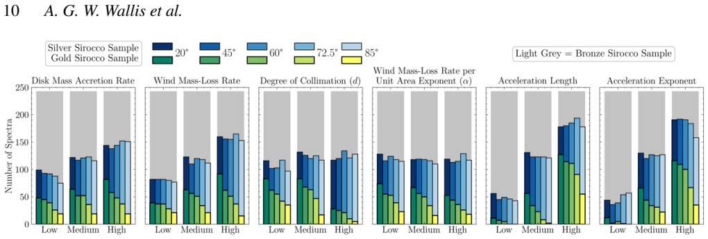
Figures from the paper (7 more)



Forward citations
Cited by 1 Pith paper
-
How massive and clumpy must a quasar wind be to create emission line blueshifts?
Blueshifted C IV emission in quasars requires wind mass-loading ϵ_w/f_V ∼ 50, disfavouring smooth disc winds in favour of clumpy or ambient-swept outflows.
Reference graph
Works this paper leans on
-
[1]
Beristain G., Edwards S., Kwan J., 2001, @doi [The Astrophysical Journal] 10.1086/320233 , 551, 1037
doi:10.1086/320233 2001
-
[2]
Boroson T. A., Green R. F., 1992, @doi [The Astrophysical Journal Supplement Series] 10.1086/191661 , 80, 109
doi:10.1086/191661 1992
-
[3]
Cordova F. A., Mason K. O., 1982, @doi [The Astrophysical Journal] 10.1086/160291 , 260, 716
-
[4]
Czekala I., Andrews S. M., Mandel K. S., Hogg D. W., Green G. M., 2015, @doi [The Astrophysical Journal] 10.1088/0004-637X/812/2/128 , 812, 128
-
[5]
Cúneo V. A., et al., 2020, @doi [Monthly Notices of the Royal Astronomical Society] 10.1093/mnras/staa2241 , 498, 25
-
[6]
A., et al., 2023, @doi [Astronomy & Astrophysics] 10.1051/0004-6361/202347265 , 679, A85
Cúneo V. A., et al., 2023, @doi [Astronomy & Astrophysics] 10.1051/0004-6361/202347265 , 679, A85
-
[7]
Dennis B. R., Phillips K. J. H., 2024, Emission Measures Demystified , @doi 10.48550/arXiv.2403.14845 , http://arxiv.org/abs/2403.14845
work page Pith review arXiv doi:10.48550/arxiv.2403.14845 2024
-
[8]
Drew J. E., 1987, @doi [Monthly Notices of the Royal Astronomical Society] 10.1093/mnras/224.3.595 , 224, 595
Show all 62 references
-
[9]
Edwards S., Fischer W., Hillenbrand L., Kwan J., 2006, @doi [The Astrophysical Journal] 10.1086/504832 , 646, 319
2006 doi
-
[10]
Filiz Ak N., et al., 2014, @doi [The Astrophysical Journal] 10.1088/0004-637X/791/2/88 , 791, 88
2014 doi
-
[11]
J., 2002, Accretion Power in Astrophysics, p
Frank J., King A., Raine D. J., 2002, Accretion Power in Astrophysics, p. 398
2002
-
[12]
S., 2004, Observations of Outflows in Cataclysmic Variables , @doi 10.48550/arXiv.astro-ph/0410200 , http://arxiv.org/abs/astro-ph/0410200
Froning C. S., 2004, Observations of Outflows in Cataclysmic Variables , @doi 10.48550/arXiv.astro-ph/0410200 , http://arxiv.org/abs/astro-ph/0410200
-
[13]
D., O'brien T
Gill C. D., O'brien T. J., 1999, @doi [Monthly Notices of the Royal Astronomical Society] 10.1046/j.1365-8711.1999.02681.x , 307, 677
1999
-
[14]
H., Di Stefano R., Prestwich A., González-Riestra R., Szentasko L., Chavarría C., 1999, @doi [Astronomy and Astrophysics] 10.48550/arXiv.astro-ph/9812054 , 343, 183
Greiner J., Tovmassian G. H., Di Stefano R., Prestwich A., González-Riestra R., Szentasko L., Chavarría C., 1999, @doi [Astronomy and Astrophysics] 10.48550/arXiv.astro-ph/9812054 , 343, 183
-
[15]
J., Rutten R
Groot P. J., Rutten R. G. M., van Paradijs J., 2004, @doi [Astronomy and Astrophysics] 10.1051/0004-6361:20031771 , 417, 283
2004 doi
-
[16]
B., et al., 2002, @doi [The Astrophysical Journal Supplement Series] 10.1086/340546 , 141, 267
Hall P. B., et al., 2002, @doi [The Astrophysical Journal Supplement Series] 10.1086/340546 , 141, 267
2002 doi
-
[17]
R., et al., 2020, @doi [Nature] 10.1038/s41586-020-2649-2 , 585, 357
Harris C. R., et al., 2020, @doi [Nature] 10.1038/s41586-020-2649-2 , 585, 357
2020 doi
-
[18]
E., Drew J
Hartley L. E., Drew J. E., Long K. S., Knigge C., Proga D., 2002, @doi [Monthly Notices of the Royal Astronomical Society] 10.1046/j.1365-8711.2002.05277.x , 332, 127
2002
-
[19]
R., et al., 1978, @doi [Nature] 10.1038/275385a0 , 275, 385
Heap S. R., et al., 1978, @doi [Nature] 10.1038/275385a0 , 275, 385
1978 doi
-
[20]
V., Panek R
Holm A. V., Panek R. J., Schiffer Iii F. H., 1982, @doi [The Astrophysical Journal] 10.1086/183714 , 252, L35
1982 doi
-
[21]
K., Kafka S., Robertson J
Honeycutt R. K., Kafka S., Robertson J. W., 2013, @doi [The Astronomical Journal] 10.1088/0004-6256/145/2/45 , 145, 45
2013 doi
-
[22]
R., 1986, @doi [Monthly Notices of the Royal Astronomical Society] 10.1093/mnras/218.4.761 , 218, 761
Horne K., Marsh T. R., 1986, @doi [Monthly Notices of the Royal Astronomical Society] 10.1093/mnras/218.4.761 , 218, 761
1986 doi
-
[23]
D., 2007, @doi [Computing in Science & Engineering] 10.1109/MCSE.2007.55 , 9, 90
Hunter J. D., 2007, @doi [Computing in Science & Engineering] 10.1109/MCSE.2007.55 , 9, 90
2007 doi
-
[24]
E., 1997, @doi [The Astrophysical Journal] 10.1086/304519 , 486, 445
Knigge C., Drew J. E., 1997, @doi [The Astrophysical Journal] 10.1086/304519 , 486, 445
1997 doi
-
[25]
A., Drew J
Knigge C., Woods J. A., Drew J. E., 1995, @doi [Monthly Notices of the Royal Astronomical Society] 10.1093/mnras/273.2.225 , 273, 225
1995 doi
-
[26]
S., Blair W
Knigge C., Long K. S., Blair W. P., Wade R. A., 1997, @doi [The Astrophysical Journal] 10.1086/303607 , 476, 291
1997 doi
-
[27]
La Dous C., 1990, @doi [Space Science Reviews] 10.1007/BF00167124 , 52, 203
1990 doi
-
[28]
M., Moore J
Leighly K. M., Moore J. R., 2004, @doi [The Astrophysical Journal] 10.1086/422088 , 611, 107
2004 doi
-
[29]
P., Szkody P., Gänsicke B., Long K
Linnell A. P., Szkody P., Gänsicke B., Long K. S., Sion E. M., Hoard D. W., Hubeny I., 2005, @doi [The Astrophysical Journal] 10.1086/429143 , 624, 923
2005 doi
-
[30]
Mata Sánchez D., et al., 2018, @doi [Monthly Notices of the Royal Astronomical Society] 10.1093/mnras/sty2402 , 481, 2646
2018 doi
-
[31]
Mata Sánchez D., et al., 2022, Hard-state optical wind during the discovery outburst of the black-hole X -ray dipper MAXI J1803 -298, @doi 10.48550/arXiv.2201.09896 , http://arxiv.org/abs/2201.09896
2022 doi
-
[32]
Mata Sánchez D., Muñoz-Darias T., Casares J., Huertas-Company M., Panizo-Espinar G., 2023, @doi [Monthly Notices of the Royal Astronomical Society] 10.1093/mnras/stad1895 , 524, 338
2023 doi
-
[33]
Matthews J., 2016, phd, University of Southampton, https://eprints.soton.ac.uk/400903/
2016
-
[34]
H., Knigge C., Long K
Matthews J. H., Knigge C., Long K. S., Sim S. A., Higginbottom N., 2015, @doi [Monthly Notices of the Royal Astronomical Society] 10.1093/mnras/stv867 , 450, 3331
2015 doi
-
[35]
H., Knigge C., Long K
Matthews J. H., Knigge C., Long K. S., Sim S. A., Higginbottom N., Mangham S. W., 2016, @doi [Monthly Notices of the Royal Astronomical Society] 10.1093/mnras/stw323 , 458, 293
2016 doi
-
[36]
H., Knigge C., Higginbottom N., Long K
Matthews J. H., Knigge C., Higginbottom N., Long K. S., Sim S. A., Mangham S. W., Parkinson E. J., Hewitt H. A., 2020, @doi [Monthly Notices of the Royal Astronomical Society] 10.1093/mnras/staa136 , 492, 5540
2020 doi
-
[37]
H., et al., 2023, @doi [Monthly Notices of the Royal Astronomical Society] 10.1093/mnras/stad2895 , 526, 3967
Matthews J. H., et al., 2023, @doi [Monthly Notices of the Royal Astronomical Society] 10.1093/mnras/stad2895 , 526, 3967
2023 doi
-
[38]
H., et al., 2024, SIROCCO : A Publicly Available Monte Carlo Ionization and Radiative Transfer Code for Astrophysical Outflows , http://arxiv.org/abs/2410.19908
Matthews J. H., et al., 2024, SIROCCO : A Publicly Available Monte Carlo Ionization and Radiative Transfer Code for Astrophysical Outflows , http://arxiv.org/abs/2410.19908
2024 arXiv
-
[39]
M., Shields J
McGraw S. M., Shields J. C., Hamann F. W., Capellupo D. M., Herbst H., 2018, @doi [Monthly Notices of the Royal Astronomical Society] 10.1093/mnras/stx3219 , 475, 585
2018 doi
-
[40]
M., Raymond J., Reynolds C
Miller J. M., Raymond J., Reynolds C. S., Fabian A. C., Kallman T. R., Homan J., 2008, @doi [The Astrophysical Journal] 10.1086/588521 , 680, 1359
2008 doi
-
[41]
Muñoz-Darias T., et al., 2019, @doi [The Astrophysical Journal Letters] 10.3847/2041-8213/ab2768 , 879, L4
2019 doi
-
[42]
Muñoz-Darias T., et al., 2020, @doi [The Astrophysical Journal] 10.3847/2041-8213/ab8381 , 893, L19
2020 doi
-
[43]
Panizo-Espinar G., Muñoz-Darias T., Armas Padilla M., Jiménez-Ibarra F., Casares J., Mata Sánchez D., 2021, @doi [Astronomy & Astrophysics] 10.1051/0004-6361/202140323 , 650, A135
2021 doi
- [44]
-
[45]
R., Fried R., Skillman D
Patterson J., Thorstensen J. R., Fried R., Skillman D. R., Cook L. M., Jensen L., 2001, @doi [Publications of the Astronomical Society of the Pacific] 10.1086/317973 , 113, 72
2001 doi
-
[46]
Pedregosa F., et al., 2011, Journal of Machine Learning Research, 12, 2825
2011
-
[47]
K., Rosen R., 1995, @doi [Monthly Notices of the Royal Astronomical Society] 10.1093/mnras/273.2.461 , 273, 461
Prinja R. K., Rosen R., 1995, @doi [Monthly Notices of the Royal Astronomical Society] 10.1093/mnras/273.2.461 , 273, 461
1995 doi
-
[48]
K., Long K
Prinja R. K., Long K. S., Froning C. S., Knigge C., Witherick D. K., Clark J. S., Ringwald F. A., 2003, @doi [Monthly Notices of the Royal Astronomical Society] 10.1046/j.1365-8711.2003.06307.x , 340, 551
2003
-
[49]
T., Vanden Berk D
Richards G. T., Vanden Berk D. E., Reichard T. A., Hall P. B., Schneider D. P., SubbaRao M., Thakar A. R., York D. G., 2002, @doi [The Astronomical Journal] 10.1086/341167 , 124, 1
2002 doi
-
[50]
A., Naylor T., 1998, @doi [The Astronomical Journal] 10.1086/300192 , 115, 286
Ringwald F. A., Naylor T., 1998, @doi [The Astronomical Journal] 10.1086/300192 , 115, 286
1998 doi
-
[51]
Ritter H., Kolb U., 2003, @doi [Astronomy & Astrophysics] 10.1051/0004-6361:20030330 , 404, 301
2003 doi
-
[52]
Scepi N., Lesur G., Dubus G., Flock M., 2018, @doi [Astronomy and Astrophysics] 10.1051/0004-6361/201833921 , 620, A49
2018 doi
-
[53]
C., et al., 2022, @doi [Nature] 10.1038/s41586-021-04324-2 , 603, 52
Segura N. C., et al., 2022, @doi [Nature] 10.1038/s41586-021-04324-2 , 603, 52
2022 doi
-
[54]
R., Patterson J., Thorstensen J
Skillman D. R., Patterson J., Thorstensen J. R., 1995, @doi [Publications of the Astronomical Society of the Pacific] 10.1086/133590 , 107, 545
1995 doi
-
[55]
Smak J., 1981, Acta Astronomica, 31, 395
1981
- [56]
-
[57]
M., Kaastra J., Zoghbi A., Kallman A
Trueba N., Miller J. M., Kaastra J., Zoghbi A., Kallman A. C. F. T., Proga D., Raymond J., 2019, @doi [The Astrophysical Journal] 10.3847/1538-4357/ab4f70 , 886, 104
2019 doi
-
[58]
Virtanen P., et al., 2020, @doi [Nature Methods] 10.1038/s41592-019-0686-2 , 17, 261
2020 doi
-
[59]
Vitello P., Shlosman I., 1993, @doi [The Astrophysical Journal] 10.1086/172799 , 410, 815
1993 doi
-
[60]
J., Morris S
Weymann R. J., Morris S. L., Foltz C. B., Hewett P. C., 1991, @doi [The Astrophysical Journal] 10.1086/170020 , 373, 23
1991 doi
- [61]
-
[62]
write newline
" write newline "" before.all 'output.state := FUNCTION fin.entry write newline FUNCTION new.block output.state before.all = 'skip after.block 'output.state := if FUNCTION new.sentence output.state after.block = 'skip output.state before.all = 'skip after.sentence 'output.stat...
Reviewed August 5, 2026 · model on record in the stance chip above.
Discussion (0). Sign in to comment.