Improving Generative Methods for Causal Evaluation via Simulation-Based Inference

Amit Sharma; David Jensen; Pracheta Amaranath; Vinitra Muralikrishnan

arxiv: 2509.02892 · v2 · submitted 2025-09-02 · 💻 cs.LG · stat.ME

Improving Generative Methods for Causal Evaluation via Simulation-Based Inference

Pracheta Amaranath , Vinitra Muralikrishnan , Amit Sharma , David Jensen This is my paper

Pith reviewed 2026-05-18 18:56 UTC · model grok-4.3

classification 💻 cs.LG stat.ME

keywords simulation-based inferencecausal estimationsynthetic data generationgenerative modelscausal evaluationposterior inferenceestimator comparisonobservational data

0 comments

The pith

SBICE uses simulation-based inference to infer distributions over generative methods and parameters from source data, creating synthetic datasets whose causal estimates align with the original.

A machine-rendered reading of the paper's core claim, the machinery that carries it, and where it could break.

The paper presents SBICE, a framework that applies simulation-based inference to select and tune generative methods for creating synthetic datasets used in causal estimator evaluation. Rather than requiring fixed choices of methods and parameter values, the approach treats these as uncertain and learns posterior distributions conditioned on the observed source dataset. This produces varied synthetic data that preserves key statistical and causal properties of the real data. A sympathetic reader would care because arbitrary choices in current generative setups can lead to misleading comparisons among causal methods. If the framework succeeds, evaluations become more robust by incorporating uncertainty and ensuring closer matches to real-world causal behavior.

Core claim

SBICE is a framework that treats the choice of generative method and its parameters as uncertain quantities. It applies simulation-based inference techniques to infer the posterior distribution of these quantities given a source dataset. The resulting posterior enables generation of synthetic datasets whose causal estimates closely match those obtained from the source data, supporting more reliable comparisons among causal estimators.

What carries the argument

Simulation-based inference for causal evaluation (SBICE), which infers posteriors over generative methods and parameters to generate synthetic data aligned with source causal estimates.

If this is right

Users can express and propagate uncertainty over both generative methods and parameter values instead of using fixed point estimates.
Synthetic datasets vary in aspects such as treatment effect and confounding bias while remaining anchored to the observed data distribution.
Estimator evaluations gain reliability because the generated data produces causal estimates that align with those from the source.
Posterior inference over suitable generative configurations becomes feasible, avoiding reliance on single deterministic choices.

Where Pith is reading between the lines

These are editorial extensions of the paper, not claims the author makes directly.

The same posterior-inference approach to generative selection could apply to simulation-based evaluation in other machine learning tasks beyond causal estimation.
SBICE suggests a path toward automated, data-driven calibration of simulation parameters in causal studies where manual tuning is common.
Extending the framework to sequential or multi-source observational data might allow more flexible matching across different real-world settings.

Load-bearing premise

That simulation-based inference applied to the source dataset can reliably identify generative methods and parameter distributions whose produced synthetic data match the source in causal structure and statistical properties.

What would settle it

An experiment in which causal estimates computed on SBICE-generated synthetic datasets systematically differ from those on the source dataset would falsify the alignment claim.

Figures

Figures reproduced from arXiv: 2509.02892 by Amit Sharma, David Jensen, Pracheta Amaranath, Vinitra Muralikrishnan.

**Figure 1.** Figure 1: Simulation-based inference for causal evaluation (SBICE) To address this issue, we advocate for generative methods that represent DGP parameters not as fixed values but as distributions that reflect user uncertainty. This perspective enables a more expressive form of sensitivity analysis, where identifiability of causal effects is treated as a continuum: users can encode varying degrees of uncertainty ove… view at source ↗

**Figure 2.** Figure 2: Boxplots of the bias (estimated ATE − true ATE) for a set of causal estimators for all generative methods across three different settings for the Lalonde (Observational) dataset. We note that estimators are inconsistent across different settings and generative methods, emphasizing the impact of setting the right DGP parameter in the generative method. FrugalFlows [de Vassimon Manela et al., 2024] paper (la… view at source ↗

**Figure 3.** Figure 3: Variation in estimator bias across different values of ρ (representing unobserved confounding) for Frugal DGP2 generated using FrugalFlows. Estimators such as TMLE and Doubly Robust (Linear) show greater sensitivity to unobserved confounding than others. Key Takeaway: Our analysis shows that while generative methods enable controlled variation in the data-generating process, differences in how methods e… view at source ↗

**Figure 4.** Figure 4: We plot the BSE for a set of causal estimators for the datasets in Table 2. Lower BSE values [PITH_FULL_IMAGE:figures/full_fig_p009_4.png] view at source ↗

**Figure 5.** Figure 5: Classifier AUC and Mean BSE of causal estimators for DGP: LinearParam DGP1 and [PITH_FULL_IMAGE:figures/full_fig_p019_5.png] view at source ↗

**Figure 6.** Figure 6: Posterior distribution for DGP: LinearParam DGP1, Simulator: LinearParam Sim1 [PITH_FULL_IMAGE:figures/full_fig_p019_6.png] view at source ↗

**Figure 7.** Figure 7: Classifier AUC and Mean BSE of causal estimators for DGP: LinearParam DGP1 and [PITH_FULL_IMAGE:figures/full_fig_p020_7.png] view at source ↗

**Figure 8.** Figure 8: Posterior distribution for DGP: LinearParam DGP1, Simulator: LinearParam Sim2 [PITH_FULL_IMAGE:figures/full_fig_p020_8.png] view at source ↗

**Figure 9.** Figure 9: Classifier AUC and Mean BSE of causal estimators for DGP: LinearParam DGP1 and [PITH_FULL_IMAGE:figures/full_fig_p021_9.png] view at source ↗

**Figure 10.** Figure 10: Posterior distribution for DGP: LinearParam DGP1, Simulator: LinearParam Sim3 [PITH_FULL_IMAGE:figures/full_fig_p021_10.png] view at source ↗

**Figure 11.** Figure 11: Classifier AUC and Mean BSE of causal estimators for DGP: LinearParam DGP1 and [PITH_FULL_IMAGE:figures/full_fig_p021_11.png] view at source ↗

**Figure 12.** Figure 12: Posterior distribution for DGP: LinearParam DGP1, Simulator: LinearParam Sim4 [PITH_FULL_IMAGE:figures/full_fig_p022_12.png] view at source ↗

**Figure 13.** Figure 13: Classifier AUC and Mean BSE of causal estimators for DGP: LinearParam DGP5 and [PITH_FULL_IMAGE:figures/full_fig_p022_13.png] view at source ↗

**Figure 14.** Figure 14: Posterior distribution for DGP: LinearParam DGP5, Simulator: LinearParam Sim1 [PITH_FULL_IMAGE:figures/full_fig_p023_14.png] view at source ↗

**Figure 15.** Figure 15: Classifier AUC and Mean BSE of causal estimators for DGP: LinearParam DGP6 and [PITH_FULL_IMAGE:figures/full_fig_p024_15.png] view at source ↗

**Figure 16.** Figure 16: Posterior distribution for DGP: LinearParam DGP6, Simulator: LinearParam Sim6 [PITH_FULL_IMAGE:figures/full_fig_p024_16.png] view at source ↗

**Figure 17.** Figure 17: Classifier AUC and Mean BSE of causal estimators for DGP: LinearParam DGP6 and [PITH_FULL_IMAGE:figures/full_fig_p025_17.png] view at source ↗

**Figure 18.** Figure 18: Posterior distribution for DGP: LinearParam DGP6, Simulator: LinearParam Sim7 (similar [PITH_FULL_IMAGE:figures/full_fig_p025_18.png] view at source ↗

**Figure 19.** Figure 19: Classifier AUC and mean BSE of causal estimators for DGP: LinearParam DGP8 and [PITH_FULL_IMAGE:figures/full_fig_p026_19.png] view at source ↗

**Figure 20.** Figure 20: Posterior distribution for DGP: LinearParam DGP8, Simulator: LinearParam Sim8 (similar [PITH_FULL_IMAGE:figures/full_fig_p026_20.png] view at source ↗

**Figure 21.** Figure 21: Classifier AUC and Mean BSE of causal estimators for DGP: LinearParam DGP6 and [PITH_FULL_IMAGE:figures/full_fig_p027_21.png] view at source ↗

**Figure 22.** Figure 22: Posterior distribution for DGP: LinearParam DGP6, Simulator: LinearParam Sim9 [PITH_FULL_IMAGE:figures/full_fig_p027_22.png] view at source ↗

**Figure 23.** Figure 23: Classifier AUC and Mean BSE of causal estimators for DGP: LinearParam DGP10 and [PITH_FULL_IMAGE:figures/full_fig_p028_23.png] view at source ↗

**Figure 24.** Figure 24: Posterior distribution for DGP: LinearParam DGP10, Simulator: LinearParam Sim10 [PITH_FULL_IMAGE:figures/full_fig_p028_24.png] view at source ↗

**Figure 25.** Figure 25: Classifier AUC and Mean BSE of causal estimators for DGP: FrugalParam DGP1 and [PITH_FULL_IMAGE:figures/full_fig_p031_25.png] view at source ↗

**Figure 26.** Figure 26: Classifier AUC and Mean BSE of causal estimators for DGP: Frugal DGP2 and Simulator: [PITH_FULL_IMAGE:figures/full_fig_p032_26.png] view at source ↗

**Figure 27.** Figure 27: Classifier AUC and Mean BSE of causal estimators for DGP: Frugal DGP3 and Simulator: [PITH_FULL_IMAGE:figures/full_fig_p033_27.png] view at source ↗

**Figure 28.** Figure 28: Classifier AUC and Mean BSE of causal estimators for DGP: Frugal DGP3 and Simulator: [PITH_FULL_IMAGE:figures/full_fig_p033_28.png] view at source ↗

**Figure 29.** Figure 29: Classifier AUC and Mean BSE of causal estimators for DGP: Frugal DGP4 and Simulator: [PITH_FULL_IMAGE:figures/full_fig_p034_29.png] view at source ↗

**Figure 30.** Figure 30: Classifier AUC and Mean BSE of causal estimators for DGP: Frugal DGP4 and Simulator: [PITH_FULL_IMAGE:figures/full_fig_p035_30.png] view at source ↗

**Figure 31.** Figure 31: Classifier AUC and Mean BSE of causal estimators for DGP: Frugal DGP4 and Simulator: [PITH_FULL_IMAGE:figures/full_fig_p036_31.png] view at source ↗

**Figure 32.** Figure 32: Classifier AUC and Mean BSE of causal estimators for DGP: Frugal DGP5 and Simulator: [PITH_FULL_IMAGE:figures/full_fig_p037_32.png] view at source ↗

**Figure 33.** Figure 33: Classifier AUC and Mean BSE of causal estimators for DGP: Frugal DGP5 and Simulator: [PITH_FULL_IMAGE:figures/full_fig_p038_33.png] view at source ↗

**Figure 34.** Figure 34: Classifier AUC and Mean BSE of causal estimators for DGP: Lalonde (Exp) and Simulator: [PITH_FULL_IMAGE:figures/full_fig_p039_34.png] view at source ↗

**Figure 35.** Figure 35: Bias squared error for causal estimators for the Lalonde (obs) dataset [PITH_FULL_IMAGE:figures/full_fig_p040_35.png] view at source ↗

**Figure 36.** Figure 36: Classifier AUC and Mean BSE of causal estimators for DGP: Project STAR and Simulator: [PITH_FULL_IMAGE:figures/full_fig_p041_36.png] view at source ↗

**Figure 37.** Figure 37: Classifier AUC and Mean BSE of causal estimators for DGP: Project STAR and Simulator: [PITH_FULL_IMAGE:figures/full_fig_p041_37.png] view at source ↗

**Figure 38.** Figure 38: Marginal distribution of outcome Y for LinearParam DGP11 [PITH_FULL_IMAGE:figures/full_fig_p043_38.png] view at source ↗

**Figure 39.** Figure 39: ATEs for the generated datasets across generative methods for the three different settings [PITH_FULL_IMAGE:figures/full_fig_p043_39.png] view at source ↗

**Figure 40.** Figure 40: Boxplots of the bias (estimated ATE − true ATE) for a set of causal estimators for all generative methods across three different settings for the Synthetic DGP1 dataset. 43 [PITH_FULL_IMAGE:figures/full_fig_p043_40.png] view at source ↗

**Figure 41.** Figure 41: Mean and Standard deviation of Classifier AUC scores for each method under the Learned ATE setting. Gen. method AUC Credence 1.0 ± 0.0 Modified Credence 1.0 ± 0.0 Realcause 1.0 ± 0.0 Frugal Flows 0.592 ± 0.012 [PITH_FULL_IMAGE:figures/full_fig_p044_41.png] view at source ↗

**Figure 42.** Figure 42: The Bias and Classifier AUC for learned ATE setting across all methods: Param DGP12 [PITH_FULL_IMAGE:figures/full_fig_p044_42.png] view at source ↗

**Figure 43.** Figure 43: Mean and Standard deviation of Classifier AUC scores for each method under the Learned ATE setting. Gen. method AUC Credence 1.0 ± 0.0 Modified Credence 1.0 ± 0.0 Realcause 1.0 ± 0.0 Frugal Flows 0.978 ± 0.001 [PITH_FULL_IMAGE:figures/full_fig_p045_43.png] view at source ↗

**Figure 44.** Figure 44: The bias and classifier AUC for learned ATE setting across all methods: Param DGP13 [PITH_FULL_IMAGE:figures/full_fig_p045_44.png] view at source ↗

**Figure 45.** Figure 45: Mean and Standard deviation of Classifier AUC scores for each method under the Learned ATE setting. Gen. method AUC Credence 1.0 ± 0.0 Modified Credence 1.0 ± 0.0 Realcause 1.0 ± 0.0 Frugal Flows 0.848 ± 0.006 [PITH_FULL_IMAGE:figures/full_fig_p045_45.png] view at source ↗

**Figure 46.** Figure 46: The bias and classifier AUC for learned ATE setting across all methods: Param DGP14 [PITH_FULL_IMAGE:figures/full_fig_p045_46.png] view at source ↗

**Figure 47.** Figure 47: Mean and Standard deviation of Classifier AUC scores for each method under the Learned ATE setting. Gen. method AUC Credence 1.0 ± 0.0 Modified Credence 1.0 ± 0.0 Realcause 1.0 ± 0.0 Frugal Flows 0.576 ± 0.009 [PITH_FULL_IMAGE:figures/full_fig_p046_47.png] view at source ↗

**Figure 48.** Figure 48: The bias and classifier AUC for learned ATE setting across all methods: Param DGP15 [PITH_FULL_IMAGE:figures/full_fig_p046_48.png] view at source ↗

**Figure 49.** Figure 49: Marginal distribution of outcome Y for the Lalonde (Exp) datasets [PITH_FULL_IMAGE:figures/full_fig_p047_49.png] view at source ↗

**Figure 50.** Figure 50: ATEs for the generated datasets across generative methods for the three different settings [PITH_FULL_IMAGE:figures/full_fig_p047_50.png] view at source ↗

**Figure 51.** Figure 51: Boxplots of the bias (estimated ATE − true ATE) for a set of causal estimators for all generative methods across three different settings for the Lalonde (Experimental) dataset. H.2.2 Lalonde (Obs) For the observational study, we included the classifier AUC and bias of the datasets across generative methods and settings in Section 2. Here, we supplement these results by including the marginal distribution… view at source ↗

**Figure 52.** Figure 52: Marginal distribution of outcome Y for the Lalonde (Obs) datasets [PITH_FULL_IMAGE:figures/full_fig_p048_52.png] view at source ↗

**Figure 53.** Figure 53: ATEs for the generated datasets across generative methods for the three different settings [PITH_FULL_IMAGE:figures/full_fig_p048_53.png] view at source ↗

read the original abstract

Generating synthetic datasets that accurately reflect real-world observational data is critical for evaluating causal estimators, but it remains a challenging task. Existing generative methods offer a solution by producing synthetic datasets anchored in the observed data (source data) while allowing variation in key parameters such as the treatment effect and amount of confounding bias. However, it is often unclear which generative methods to use and which values of parameters to choose when generating synthetic datasets. Moreover, existing methods typically require users to provide fixed point estimates of such parameters. This denies users the ability to express uncertainty over both generative methods and parameter values and removes the potential for posterior inference, potentially leading to unreliable estimator comparisons. We introduce simulation-based inference for causal evaluation (SBICE), a framework that treats the generative method and its corresponding generative parameters as uncertain and infers their posterior distribution given a source dataset. Leveraging techniques in simulation-based inference, SBICE identifies suitable generative methods and infers distributions over its parameter configurations to produce synthetic datasets closely aligned with the source data distribution. Empirical results demonstrate that SBICE improves the reliability of estimator evaluations by generating realistic datasets whose causal estimates closely match the estimates of the source data, making it a robust and uncertainty-aware approach to selecting causal estimators.

Editorial analysis

A structured set of objections, weighed in public.

Desk editor's note, referee report, simulated authors' rebuttal, and a circularity audit. Tearing a paper down is the easy half of reading it; the pith above is the substance, this is the friction.

Desk Editor's Note private letter to a colleague

SBICE applies simulation-based inference to pick generative methods and parameters for causal synthetic data, which is a reasonable fix for ad-hoc choices but rests on thin empirical detail.

read the letter

The main point is that this paper uses simulation-based inference to treat both the choice of generative method and its parameters as uncertain quantities, then infers a posterior over them from a source dataset instead of requiring users to pick fixed values by hand. That framing directly targets the arbitrariness that often creeps into synthetic data generation for causal estimator tests. What they actually do is run SBI to produce synthetic sets whose causal estimates are meant to line up with those from the real source data. The idea is sensible on its face and gives users a way to express uncertainty rather than committing to point estimates for things like treatment effect or confounding strength. It also avoids reducing the problem to a single hand-tuned configuration. The execution looks standard for SBI work: they model the generative process as the simulator and use posterior inference to match properties of the source. That part is straightforward and builds on existing tools without obvious reinvention. The soft spot is that the abstract claims empirical gains in reliability and close matching of causal estimates, yet supplies no numbers, no description of the SBI architecture, no ablation on summary statistics, and no comparison to simpler baselines like expert-specified ranges or basic grid search. Without those, it is hard to tell whether the posterior actually improves downstream estimator rankings or just adds computational overhead while recovering something close to what a careful user would have chosen anyway. The assumption that SBI can recover generative configs whose causal structure matches the source also needs concrete checks, especially on datasets with strong selection or non-linear effects. This is for people who build or rely on synthetic benchmarks in causal ML. A reader who already generates their own test data and worries about sensitivity to generative choices could try the framework and see if it changes their conclusions. It is coherent enough on its own terms to deserve a serious referee who can examine the methods section and the actual results.

Referee Report

2 major / 2 minor

Summary. The paper introduces SBICE, a framework that applies simulation-based inference to infer posterior distributions over generative methods and their parameters (such as treatment effect and confounding bias) conditioned on a source observational dataset. This enables generation of synthetic datasets for causal estimator evaluation that incorporate uncertainty rather than relying on fixed point estimates, with the central empirical claim being that the resulting datasets produce causal estimates closely matching those from the source data.

Significance. If the empirical validation holds, SBICE offers a practical advance for benchmarking causal methods by making synthetic data generation uncertainty-aware and better aligned with real data distributions. It usefully extends established SBI techniques to the causal evaluation setting and provides a reproducible path for posterior inference over generative choices, which is a clear strength relative to prior fixed-parameter approaches.

major comments (2)

[Experiments] Experimental evaluation: the claim that SBICE generates datasets 'whose causal estimates closely match the estimates of the source data' is central but requires explicit quantitative support (e.g., reported differences in ATE or CATE estimates, overlap metrics, or statistical tests between source and synthetic distributions). Without these numbers and ablations on the SBI components, the improvement in reliability cannot be fully assessed.
[Method] Method section: the procedure for selecting summary statistics in the SBI step is load-bearing for the posterior inference to recover causal structure; the manuscript should specify and justify the chosen statistics (or demonstrate robustness) because poor choice could prevent the generated data from matching the source causal properties.

minor comments (2)

[Introduction] Notation for the generative parameters (treatment effect, confounding bias) should be introduced with explicit symbols early in the methods to avoid ambiguity when describing the posterior.
Figures comparing causal estimates should include error bars or credible intervals to visually support the matching claim.

Simulated Author's Rebuttal

2 responses · 0 unresolved

We thank the referee for their constructive comments and recommendation of minor revision. We address each major comment below, providing additional quantitative support and methodological clarifications where appropriate.

read point-by-point responses

Referee: [Experiments] Experimental evaluation: the claim that SBICE generates datasets 'whose causal estimates closely match the estimates of the source data' is central but requires explicit quantitative support (e.g., reported differences in ATE or CATE estimates, overlap metrics, or statistical tests between source and synthetic distributions). Without these numbers and ablations on the SBI components, the improvement in reliability cannot be fully assessed.

Authors: We agree that explicit quantitative metrics are needed to fully support the central empirical claim. In the revised manuscript we have added a dedicated experimental subsection containing a table that reports mean absolute differences in ATE and CATE estimates between the source data and SBICE-generated synthetic datasets, together with Wasserstein distances and two-sample Kolmogorov-Smirnov p-values assessing distributional overlap. We have also included ablations that isolate the contribution of the SBI posterior inference step versus simpler point-estimate baselines. revision: yes
Referee: [Method] Method section: the procedure for selecting summary statistics in the SBI step is load-bearing for the posterior inference to recover causal structure; the manuscript should specify and justify the chosen statistics (or demonstrate robustness) because poor choice could prevent the generated data from matching the source causal properties.

Authors: We have expanded the method section to explicitly enumerate the summary statistics used (first and second moments of the joint distribution of covariates, treatment, and outcome, plus the treatment-outcome correlation and selected conditional moments). Their selection is justified by their ability to capture both marginal and dependence structure relevant to causal identification. We further added a robustness subsection that perturbs the statistic set and shows that the recovered posteriors and downstream causal estimates remain stable. revision: yes

Circularity Check

0 steps flagged

No significant circularity identified

full rationale

The paper proposes SBICE by applying established simulation-based inference methods to an external source dataset in order to infer posteriors over generative models and parameters. The central empirical claim is that the resulting synthetic datasets produce causal estimates close to those of the source data. This validation step is independent of the fitting process itself and does not reduce any claimed prediction or result to a quantity defined by the fitted parameters or by self-referential construction. No load-bearing step in the derivation chain is shown to be equivalent to its inputs by the paper's own equations or citations.

Axiom & Free-Parameter Ledger

1 free parameters · 1 axioms · 0 invented entities

The central claim depends on the applicability of simulation-based inference to select among generative models and on the assumption that matching causal estimates is a sufficient proxy for distributional alignment with the source data.

free parameters (1)

generative parameters (treatment effect, confounding bias)
These quantities are treated as uncertain and inferred rather than fixed point estimates; their posterior is central to the synthetic data generation process.

axioms (1)

domain assumption Simulation-based inference can approximate the posterior over both discrete generative method choices and continuous parameters given only the source observational dataset.
This is the core modeling assumption that enables SBICE to replace fixed-point user choices with inferred distributions.

pith-pipeline@v0.9.0 · 5753 in / 1242 out tokens · 49218 ms · 2026-05-18T18:56:40.414262+00:00 · methodology

discussion (0)

Lean theorems connected to this paper

Citations machine-checked in the Pith Canon. Every link opens the source theorem in the public Lean library.

IndisputableMonolith/Cost/FunctionalEquation.lean washburn_uniqueness_aczel unclear

?

unclear
Relation between the paper passage and the cited Recognition theorem.

We introduce simulation-based inference for causal evaluation (SBICE), a framework that models generative parameters as uncertain and infers their posterior distribution given a source dataset. Leveraging techniques in simulation-based inference, SBICE identifies parameter configurations that produce synthetic datasets closely aligned with the source data distribution.
IndisputableMonolith/Foundation/AlexanderDuality.lean alexander_duality_circle_linking unclear

?

unclear
Relation between the paper passage and the cited Recognition theorem.

We use four different generative methods: (1) Credence; (2) a modified version of Credence ... (3) Realcause; and (4) FrugalFlows.
IndisputableMonolith/Foundation/AbsoluteFloorClosure.lean absolute_floor_iff_bare_distinguishability unclear

?

unclear
Relation between the paper passage and the cited Recognition theorem.

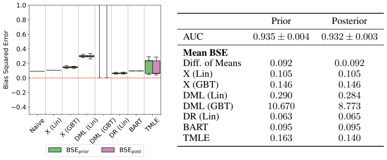
We define the mean BSE for the posterior-source datasets ... Mean BSEM;post = 1/N Σ [ (τ(i)M;post − τ∗(i)post) − (τM;source − τ∗) ]²

What do these tags mean?

matches: The paper's claim is directly supported by a theorem in the formal canon.
supports: The theorem supports part of the paper's argument, but the paper may add assumptions or extra steps.
extends: The paper goes beyond the formal theorem; the theorem is a base layer rather than the whole result.
uses: The paper appears to rely on the theorem as machinery.
contradicts: The paper's claim conflicts with a theorem or certificate in the canon.
unclear: Pith found a possible connection, but the passage is too broad, indirect, or ambiguous to say the theorem truly supports the claim.

Reference graph

Works this paper leans on

12 extracted references · 12 canonical work pages

[1]

"X y P (y|t = 1, x) # −

doi: 10.21105/joss.04304. URL https://doi.org/10.21105/joss.04304. Keith Battocchi, Eleanor Dillon, Maggie Hei, Greg Lewis, Paul Oka, Miruna Oprescu, and Vasilis Syrgkanis. EconML: A Python Package for ML-Based Heterogeneous Treatment Effects Estima- tion. https://github.com/py-why/EconML, 2019. Version 0.x. Vincent Dorie, Hugh Chipman, and Robert McCullo...

work page doi:10.21105/joss.04304 2019
[2]

We used the implementation in the EconML [Battocchi et al., 2019] package

X-Learner [Künzel et al., 2019]: A meta-learner algorithm to estimate the average treatment effect using two different underlying function: Linear regression (referred to as X (Lin)) and Gradient Boosted Trees (referred to as X (GBT)). We used the implementation in the EconML [Battocchi et al., 2019] package

work page 2019
[3]

We used the implementation in the EconML python package, and used two learners: Linear regression (DML (Lin)) and Gradient Boosted Trees (DML (GBT))

Double machine learning (DML) [Chernozhukov et al., 2019]: An algorithm that constructs a de-biased estimator of the causal parameter by using two models to estimate the residual errors. We used the implementation in the EconML python package, and used two learners: Linear regression (DML (Lin)) and Gradient Boosted Trees (DML (GBT))

work page 2019
[4]

The advantage of using this estimator is that the effect is unbiased if either model is correctly specified

Doubly robust (DR) [Dudík et al., 2014]: This estimator combines two models: one for outcome regression and another for the treatment (propensity score) to estimate the causal effect. The advantage of using this estimator is that the effect is unbiased if either model is correctly specified. We use the implementation in the EconML package and use a linear...

work page 2014
[5]

We use its R implementation [Dorie et al., 2025] in our experiments

Causal BART [Hill, 2011]: This estimator leverages Bayesian Additive Regression Trees (BART) to estimate the causal effect. We use its R implementation [Dorie et al., 2025] in our experiments

work page 2011
[6]

Targeted Maximum Likelihood Estimator (TMLE) [Van Der Laan and Rubin, 2006]: We use the implementation of TMLE as described in the package zEpid Zivich et al. [2022]. 16 Algorithm 1: SBICE: Simulation-based inference for causal evaluation Input: Source dataset D = {X, T, Y }; Prior over knobs p(θ); Causal estimators M Output: Posterior datasets D; Causal ...

work page 2006
[7]

Source datasets from the true DGP: LinearParam DGP1,

work page
[8]

Posterior datasets using parameter samples from the posterior distribution, and

work page
[9]

Evaluation We report the mean classifier AUCs for the posterior and prior datasets in Table 5

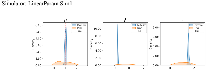
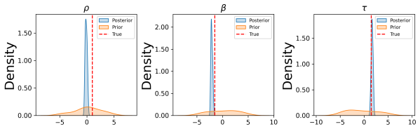
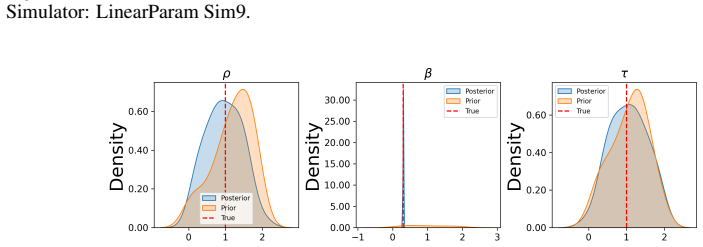
Prior datasets using parameter samples from the prior. Evaluation We report the mean classifier AUCs for the posterior and prior datasets in Table 5. We plot the bias of the causal estimators for the posterior, prior and source datasets in Figure 5. We also plot the posterior distribution for each of the DGP parameters in Figure 6. For this setting, we fi...

work page 2024
[10]

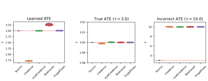
Learned ATE: We did not set any constraints to the generative method, and learned the distributions from the source data

work page
[11]

True ATE: We set the constraint that the true ATEτ = 3.0 (obtained from the data generating process)

work page
[12]

Incorrect ATE: We set the constraint that the ATEτ = 10.0 (a large, positive value compared to the ground-truth). To evaluate the differences across generative methods as well as the settings, we compared the generated datasets to the source dataset and computed the mean classifier AUC score across 50 generated datasets. The classifier AUC score for datas...

work page 2019

[1] [1]

"X y P (y|t = 1, x) # −

doi: 10.21105/joss.04304. URL https://doi.org/10.21105/joss.04304. Keith Battocchi, Eleanor Dillon, Maggie Hei, Greg Lewis, Paul Oka, Miruna Oprescu, and Vasilis Syrgkanis. EconML: A Python Package for ML-Based Heterogeneous Treatment Effects Estima- tion. https://github.com/py-why/EconML, 2019. Version 0.x. Vincent Dorie, Hugh Chipman, and Robert McCullo...

work page doi:10.21105/joss.04304 2019

[2] [2]

We used the implementation in the EconML [Battocchi et al., 2019] package

X-Learner [Künzel et al., 2019]: A meta-learner algorithm to estimate the average treatment effect using two different underlying function: Linear regression (referred to as X (Lin)) and Gradient Boosted Trees (referred to as X (GBT)). We used the implementation in the EconML [Battocchi et al., 2019] package

work page 2019

[3] [3]

We used the implementation in the EconML python package, and used two learners: Linear regression (DML (Lin)) and Gradient Boosted Trees (DML (GBT))

Double machine learning (DML) [Chernozhukov et al., 2019]: An algorithm that constructs a de-biased estimator of the causal parameter by using two models to estimate the residual errors. We used the implementation in the EconML python package, and used two learners: Linear regression (DML (Lin)) and Gradient Boosted Trees (DML (GBT))

work page 2019

[4] [4]

The advantage of using this estimator is that the effect is unbiased if either model is correctly specified

Doubly robust (DR) [Dudík et al., 2014]: This estimator combines two models: one for outcome regression and another for the treatment (propensity score) to estimate the causal effect. The advantage of using this estimator is that the effect is unbiased if either model is correctly specified. We use the implementation in the EconML package and use a linear...

work page 2014

[5] [5]

We use its R implementation [Dorie et al., 2025] in our experiments

Causal BART [Hill, 2011]: This estimator leverages Bayesian Additive Regression Trees (BART) to estimate the causal effect. We use its R implementation [Dorie et al., 2025] in our experiments

work page 2011

[6] [6]

Targeted Maximum Likelihood Estimator (TMLE) [Van Der Laan and Rubin, 2006]: We use the implementation of TMLE as described in the package zEpid Zivich et al. [2022]. 16 Algorithm 1: SBICE: Simulation-based inference for causal evaluation Input: Source dataset D = {X, T, Y }; Prior over knobs p(θ); Causal estimators M Output: Posterior datasets D; Causal ...

work page 2006

[7] [7]

Source datasets from the true DGP: LinearParam DGP1,

work page

[8] [8]

Posterior datasets using parameter samples from the posterior distribution, and

work page

[9] [9]

Evaluation We report the mean classifier AUCs for the posterior and prior datasets in Table 5

Prior datasets using parameter samples from the prior. Evaluation We report the mean classifier AUCs for the posterior and prior datasets in Table 5. We plot the bias of the causal estimators for the posterior, prior and source datasets in Figure 5. We also plot the posterior distribution for each of the DGP parameters in Figure 6. For this setting, we fi...

work page 2024

[10] [10]

Learned ATE: We did not set any constraints to the generative method, and learned the distributions from the source data

work page

[11] [11]

True ATE: We set the constraint that the true ATEτ = 3.0 (obtained from the data generating process)

work page

[12] [12]

Incorrect ATE: We set the constraint that the ATEτ = 10.0 (a large, positive value compared to the ground-truth). To evaluate the differences across generative methods as well as the settings, we compared the generated datasets to the source dataset and computed the mean classifier AUC score across 50 generated datasets. The classifier AUC score for datas...

work page 2019