REVIEW 4 major objections 5 minor 1 cited by
Split Conformal Prediction in the Function Space with Neural Operators
T0 review · 4 major / 5 minor · reviewed 2026-08-05 · deepseek-v4-flash
Pith's one-line read Split conformal prediction can be lifted from discretized grids to the full function space, giving neural operator predictions a finite-sample coverage guarantee under a bilipschitz discretization condition.
desk verdict The functional coverage theorem rests on an assumption that grid sampling cannot satisfy; the empirical heuristics and diagnostics are honest and potentially useful, but the headline guarantee does not hold as stated. read the letter →
The pith
A machine-rendered reading of the paper's core claim, the machinery that carries it, and where it could break.
The reading
What carries the argument
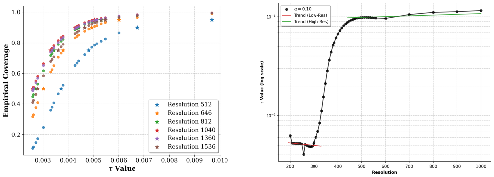
The load-bearing object is the discretization map Pd together with a quadrature-weighted L2 norm. Its key property is the bilipschitz inequality c1||u−v||Y ≤ ||Pd(u)−Pd(v)||w,2,d ≤ c2||u−v||Y, which converts a finite-dimensional split-CP threshold into a ball in the infinite-dimensional output space with radius τα/c1. The weighted norm is chosen so that the discrete score is a Riemann sum for the continuous L2 norm, giving c1 → 1 on refined grids. A heuristic additive decomposition of τα into discretization, calibration, and misspecification terms carries the resolution-transfer and super-resolution parts of the paper.
What would settle it
Construct a test set containing pairs of functions that are identical on the calibration grid but differ sharply between grid points—for example, the zero function and a narrow bump supported inside a single cell. For such pairs the discretized score is zero, so they always fall inside the calibrated set, yet their continuous L2 distance is positive; as the share of such pairs grows, empirical functional coverage drops below 1−α, demonstrating that the guarantee requires smoothness on the grid scale rather than following from grid values alone.
Extended reading notes
Core claim
The central claim is Theorem 1: for a neural operator Gθ and a discretization map Pd satisfying bilipschitz bounds c1 and c2, the functional prediction set Γα^func(f) = {v ∈ Y : ||Gθ(f) − v||Y ≤ τα/c1} satisfies P(u_{n+1} ∈ Γα^func(f_{n+1})) ≥ 1 − α, where τα is the ordinary split-CP quantile of discretized scores. The mechanism is an implication chain: the discrete event 'score below τα' entails the continuous event 'L2 distance below τα/c1', because c1||u−v||Y ≤ ||Pd(u)−Pd(v)||. The paper argues that as the grid is refined the weighted norm converges to the continuous L2 norm and c1 approaches 1, so the guaranteed radius becomes the empirically calibrated threshold itself.
Load-bearing premise
The method assumes the sampled grid captures every difference between two functions: if two solutions agree at all grid points but differ between them, the lower bilipschitz constant c1 is effectively zero and the radius τα/c1 no longer bounds the true error; the experiments simply assume c1 = 1.
Editorial extensions
If this is right
- A single scalar threshold calibrated on grid values produces a valid prediction set for whole functions, as long as the discretization is bilipschitz and c1 is known.
- The guarantee is distribution-free and finite-sample, so it does not require Gaussian or Bayesian assumptions; it applies to any exchangeable calibration set and any trained neural operator.
- The radius decomposition implies conformal thresholds shift with resolution in a predictable way, and the empirical log-linear regression transfers them to finer grids without retraining.
- Using the quadrature-weighted norm makes calibrated thresholds less sensitive to grid clustering, so the same uncertainty set remains usable across grid geometries.
- In autoregressive settings, once exchangeability is broken, the calibrated threshold no longer guarantees coverage but becomes a readable diagnostic: crossing τα flags forecast degradation in the same units as the original bound.
Reading between the lines
- Editorial inference: the discretize-then-lift proof structure is not tied to the L2 norm; any nonconformity metric with a bilipschitz projection should yield an analogous functional set, so choosing a norm aligned with the target error could give tighter or more meaningful sets.
- Editorial inference: the paper's experiments set c1 = 1 while Theorem 1 requires it to be known; a conservative variant would estimate c1 from validation pairs and inflate the radius by 1/c1, at the cost of wider sets.
- Editorial inference: the super-resolution regression is a heuristic, and its failure mode is already visible in the Poisson case; a natural test is to identify where the log-linear model of τα breaks down and replace it with a piecewise or uncertainty-aware fit.
- Editorial inference: Theorem 2's total-variation bound implies one could monitor an empirical surrogate of dTV online and issue an early warning when it approaches α, turning the binary within-τα check into a continuous safety signal.
Editorial analysis
A structured set of objections, weighed in public.
Referee Report
Summary. The paper proposes a split-conformal framework for function-valued outputs of neural operators. It introduces a quadrature-weighted L2 norm, assumes a bilipschitz discretization map between the function space and its grid evaluation, and proves Theorem 1 giving a finite-sample coverage guarantee in the function space. It then proposes a log-linear heuristic to transfer conformal radii across resolutions, and two diagnostics (CES and IA) for autoregressive forecasting. Experiments are reported on Darcy flow, 2D Poisson, and 2D Navier-Stokes, including resolution-shift and super-resolution ablations.
Significance. If the central theorem were valid, the paper would be a notable step toward uncertainty quantification for neural operators in infinite-dimensional settings. The empirical study is substantial, the code is available, and the resolution-transport heuristic plus the CES/IA diagnostics are falsifiable and potentially useful. However, the main theoretical guarantee is not established because Assumption 1 is not satisfied by grid evaluation on an infinite-dimensional space, and the implementation uses a different nonconformity score than the theorem. The paper could be made sound by re-scoping the theoretical claims to the discretized space and presenting the continuous-space result as a heuristic/asymptotic statement.
major comments (4)
- [Theoretical Foundation, Assumption 1 (Eq. 3)] The lower bound c1||u-v||_Y <= ||P_d(u)-P_d(v)||_{w,2,d} is false for grid-evaluation maps on an infinite-dimensional space. Take any grid cell and a smooth bump phi supported strictly inside that cell, with u=phi and v=0. Then P_d(u)=P_d(v), so the discrete distance is 0, while ||u-v||_Y>0. Hence no positive c1 exists. Theorem 1's proof (Appendix, Steps 2-3) uses this lower bound to pass from s_{n+1} <= tau_alpha to the continuous norm bound; the central coverage guarantee therefore does not follow. The counterexample persists for every fixed grid, so the asymptotic remark c1->1 as d->infty cannot rescue the finite-sample claim.
- [Methodology, 'Conformal Calibration' vs. Appendix Eq. (14)] The empirical score is s_i = ||hat u_i - u_i||_{w,2} / ||hat u_i||_{w,2}, and the prediction set in Eq. (9) is stated in relative error. Theorem 1 and its proof use the absolute score ||P_d(hat u_i)-P_d(u_i)||_{w,2,d} and the absolute ball in Eq. (4). No argument shows that the relative-score set inherits the coverage guarantee; the events are not equivalent without a uniform norm-ratio bound. The reported coverage numbers therefore do not validate Theorem 1's functional set.
- [Methodology, 'Conformal Calibration'] After Eq. (9) the text states 'we assume c1 = 1, following Remark 1'. Even if Assumption 1 held on a restricted class, c1 is unknown and typically <=1. Setting c1=1 makes the implemented prediction set smaller than the set tau_alpha/c1 required by the proof, so the implementation is not covered by Theorem 1. No estimate or bound for c1 is given, and the finite-sample guarantee needs c1 to be known or controlled.
- [Appendix, Additional Theoretical Results, Theorem 3] The proof of Theorem 3 is circular: Step 3 says 'Invoking Theorem 3' and 'all conditions for Theorem 3 are met' while Theorem 3 is the result being proved. The theorem statement defines Gamma_alpha(f) = {v: P(v) in hat Gamma_alpha(f)}, but the proof constructs Gamma_func_alpha = {v: ||hat u - v||_Y <= tau_alpha/c1}; these sets are not shown to coincide. The claimed delta -> 0 behavior is not derived. This theorem is therefore unsupported as stated.
minor comments (5)
- [A Heuristic Model, Eq. (7)] The notation switches between d (number of evaluation points) and R in the regression. Clarify that R denotes the resolution used in the log-linear fit.
- [Table 1 caption] 'overly consecrative coverage' should read 'overly conservative coverage'.
- [Appendix, Proof of Theorem 3] The proof begins 'he key is to formalize'; the initial 'T' is missing. Also, internal references to 'Theorem 3' in Steps 2-4 should refer to Theorem 1 if that is the intended argument.
- [Appendix, Theorem 4] The notation P_d is used both for the discretization operator and, in Theorem 4, for a sequence of partitions. Use a distinct symbol (e.g., call the partitions P^{(d)} or Q_d) to avoid confusion.
- [Super Resolution] The sentence 'described in Section .' has an empty cross-reference; fill in the section number.
Circularity Check
Auxiliary Theorem 3's proof invokes itself and Lemma 1 restates Assumption 1, but the central Theorem 1 derivation is conditionally valid and not circular.
-
other
[Appendix, Detailed Proof of Theorem 3, Step 3]
"Step 3: Invoking Theorem 3. ... Since the bilipschitz condition holds for the relevant functions (the true solutions and their approximations), all conditions for Theorem 3 are met. We calibrate a threshold τα in the discrete space as per Step 1 of the proof of Theorem 3. Then, following Steps 2-4 of that proof, we can construct a functional prediction set:"
The proof of Theorem 3 establishes its conclusion by assuming Theorem 3 itself. Step 3 is literally titled 'Invoking Theorem 3' and states 'all conditions for Theorem 3 are met,' then says it will 'follow[...] Steps 2-4 of that proof.' This means the theorem being proved is used as its own justification. No independent derivation of the functional coverage guarantee is supplied; the argument reduces to the theorem's statement. This is circular reasoning, regardless of whether the claimed result might be true.
-
renaming known result
[Appendix, Lemma 1 (Projection Stability)]
"Suppose that there exist constants c1, c2 > 0 such that for all u, v ∈ Y, c1∥u − v∥Y ≤ ∥P (u) − P (v)∥Rd ≤ c2∥u − v∥Y . Then P is bilipschitz on Y, up to the constants c1 and c2."
Lemma 1's assumption is exactly the bilipschitz inequality, and its conclusion is the same inequality relabeled as 'bilipschitz.' The proof only restates the assumption: 'The assumed double inequality implies that P preserves distances in Y up to multiplicative factors c1 and c2.' Thus the lemma adds no independent content and cannot serve as independent support for subsequent results; it is Assumption 1 repackaged as a derived stability property.
full rationale
The central derivation, Theorem 1, is not circular: the discrete split-CP guarantee P(s_{n+1} ≤ τα) ≥ 1−α is combined with the assumed lower Lipschitz bound c1∥u−v∥Y ≤ ∥Pd(u)−Pd(v)∥ to obtain the functional ball of radius τα/c1. This is a valid conditional implication; τα is a standard conformal quantile, and no fitted parameter is disguised as a prediction. The implementation later uses a relative score and sets c1=1, which is a mismatch with Theorem 1's assumptions—a correctness concern, not circularity. The super-resolution correction (Eq. 7) is explicitly labeled a heuristic with 'no formal coverage guarantee'; fitting a log-linear curve to calibration thresholds and extrapolating to a held-out resolution is an empirical prediction, and the paper does not show that the target coverage is used as an input to the fit. The genuine circular steps are confined to the appendix: Theorem 3's proof invokes Theorem 3 itself, and Lemma 1 merely restates Assumption 1. These auxiliary items do not undermine the main theorem's conditional validity, so the overall circularity score is moderate rather than high.
Assumptions & free parameters
free parameters (3)
- Bilipschitz constant c1 =
1 (assumed)
- Super-resolution regression slope s =
fitted, value not stated
- Super-resolution regression intercept b =
fitted, value not stated
assumptions (4)
- ad hoc to paper Assumption 1: Discretization map Pd is bilipschitz with constants 0 < c1 ≤ 1 ≤ c2 (Eq. 3).
- domain assumption Target functions u lie in a Sobolev space H^s with s > d/2.
- standard math Calibration and test data are i.i.d. exchangeable.
- standard math Riemann integrability of the squared solution for quadrature convergence.
Cite this review
Pith. "Pith review of Split Conformal Prediction in the Function Space with Neural Operators." pith.science (2026). https://pith.science/paper/A2BWLH66
@misc{pith2026250904623,
  author       = {Pith},
  title        = {Pith review of: Split Conformal Prediction in the Function Space with Neural Operators},
  year         = {2026},
  howpublished = {\url{https://pith.science/paper/A2BWLH66}},
  note         = {Machine review of arXiv:2509.04623}
}
read the original abstract
Uncertainty quantification for neural operators remains an open problem in the infinite-dimensional setting due to the lack of finite-sample coverage guarantees over functional outputs. While conformal prediction offers finite-sample guarantees in finite-dimensional spaces, it does not directly extend to function-valued outputs. Existing approaches (Gaussian processes, Bayesian neural networks, and quantile-based operators) require strong distributional assumptions or yield conservative coverage. This work extends split conformal prediction to function spaces following a two step method. We first establish finite-sample coverage guarantees in a finite-dimensional space using a discretization map in the output function space. Then these guarantees are lifted to the function-space by considering the asymptotic convergence as the discretization is refined. To characterize the effect of resolution, we decompose the conformal radius into discretization, calibration, and misspecification components. This decomposition motivates a regression-based correction to transfer calibration across resolutions. Additionally, we propose two diagnostic metrics (conformal ensemble score and internal agreement) to quantify forecast degradation in autoregressive settings. Empirical results show that our method maintains calibrated coverage with less variation under resolution shifts and achieves better coverage in super-resolution tasks.
Figures


Figures from the paper (6 more)




Forward citations
Cited by 1 Pith paper
-
Geometry-Aware Uncertainty Quantification via Conformal Prediction on Manifolds
Adaptive geodesic conformal prediction builds manifold-valued prediction regions with geodesic distances and a cross-validated difficulty estimator, keeping marginal coverage valid while making conditional coverage mo...
Reference graph
Works this paper leans on
-
[1]
, " * write output.state after.block = add.period write newline
ENTRY address archivePrefix author booktitle chapter edition editor eid eprint howpublished institution isbn journal key month note number organization pages publisher school series title type volume year label extra.label sort.label short.list INTEGERS output.state before.all mid.sentence after.sentence after.block FUNCTION init.state.consts #0 'before.a...
-
[2]
write newline
" write newline "" before.all 'output.state := FUNCTION n.dashify 't := "" t empty not t #1 #1 substring "-" = t #1 #2 substring "--" = not "--" * t #2 global.max substring 't := t #1 #1 substring "-" = "-" * t #2 global.max substring 't := while if t #1 #1 substring * t #2 global.max substring 't := if while FUNCTION word.in bbl.in capitalize " " * FUNCT...
-
[3]
Akhare, D.; Luo, T.; and Wang, J.-X. 2023. DiffHybrid- UQ : Uncertainty Quantification for Differentiable Hybrid Neural Modeling. arXiv:2401.00161
work page Pith review arXiv 2023
-
[4]
Baheri, A.; and Shahbazi, M. A. 2025. Multi-Scale Conformal Prediction: A Theoretical Framework with Coverage Guarantees. arXiv preprint arXiv:2502.05565
work page Pith review arXiv 2025
-
[5]
Bahmani, B.; Goswami, S.; Kevrekidis, I. G.; and Shields, M. D. 2025. A resolution independent neural operator. Computer Methods in Applied Mechanics and Engineering, 444: 118113
work page 2025
-
[6]
Barber, R. F.; Cand \`e s, E. J.; Ramdas, A.; and Tibshirani, R. J. 2023. Conformal prediction beyond exchangeability . The Annals of Statistics, 51(2): 816 -- 845
work page 2023
-
[7]
Brofos, J.; Shu, R.; and Lederman, R. R. 2019. A bias-variance decomposition for Bayesian deep learning. In NeurIPS 2019 Workshop on Bayesian Deep Learning
work page 2019
-
[8]
B \"u lte, C.; Horat, N.; Quinting, J.; and Lerch, S. 2025. Uncertainty quantification for data-driven weather models. Artificial Intelligence for the Earth Systems
work page 2025
Show all 39 references
-
[9]
J.; and Lindemann, L
Cleaveland, M.; Lee, I.; Pappas, G. J.; and Lindemann, L. 2024. Conformal prediction regions for time series using linear complementarity programming. In Proceedings of the AAAI Conference on Artificial Intelligence, volume 38, 20984--20992
2024
-
[10]
Durasov, N.; Bagautdinov, T.; Baque, P.; and Fua, P. 2021. Masksembles for uncertainty estimation. In Proceedings of the IEEE/CVF Conference on Computer Vision and Pattern Recognition, 13539--13548
2021
-
[11]
L.; Baltatzis, V.; Desai, S.; Devaraj, A.; Ellis, S.; Manzanera, O
Folgoc, L. L.; Baltatzis, V.; Desai, S.; Devaraj, A.; Ellis, S.; Manzanera, O. E. M.; Nair, A.; Qiu, H.; Schnabel, J.; and Glocker, B. 2021. Is MC dropout bayesian? arXiv preprint arXiv:2110.04286
2021 arXiv
-
[12]
Fontana, M.; Zeni, G.; and Vantini, S. 2023. Conformal prediction: A unified review of theory and new challenges . Bernoulli, 29(1): 1 -- 23
2023
-
[13]
Furuya, T.; Taniguchi, K.; and Okuda, S. 2024. Quantitative Approximation for Neural Operators in Nonlinear Parabolic Equations. arXiv preprint arXiv:2410.02151
2024 arXiv
-
[14]
Ghosh, S.; Shi, Y.; Belkhouja, T.; Yan, Y.; Doppa, J.; and Jones, B. 2023. Probabilistically robust conformal prediction. In Evans, R. J.; and Shpitser, I., eds., Proceedings of the Thirty-Ninth Conference on Uncertainty in Artificial Intelligence, volume 216 of Proceedings of...
2023
-
[15]
Goan, E.; and Fookes, C. 2020. Bayesian Neural Networks: An Introduction and Survey, 45--87. Cham: Springer International Publishing. ISBN 978-3-030-42553-1
2020
-
[16]
Guo, L.; Wu, H.; Wang, Y.; Zhou, W.; and Zhou, T. 2024. IB-UQ: Information bottleneck based uncertainty quantification for neural function regression and neural operator learning. Journal of Computational Physics, 510: 113089
2024
-
[17]
H.; and Friedman, J
Hastie, T.; Tibshirani, R.; Friedman, J. H.; and Friedman, J. H. 2009. The elements of statistical learning: data mining, inference, and prediction, volume 2. Springer
2009
-
[18]
Haussler, D.; and Warmuth, M. 2018. The probably approximately correct (PAC) and other learning models. The Mathematics of Generalization, 17--36
2018
-
[19]
E.; and Zingg, D
Hicken, J. E.; and Zingg, D. W. 2013. Summation-by-parts operators and high-order quadrature. Journal of Computational and Applied Mathematics, 237(1): 111--125
2013
-
[20]
Huang, X.; Shi, L.; and Suykens, J. A. 2013. Support vector machine classifier with pinball loss. IEEE transactions on pattern analysis and machine intelligence, 36(5): 984--997
2013
-
[21]
Katende, R. 2025. Stability Analysis of Physics-Informed Neural Networks via Variational Coercivity, Perturbation Bounds, and Concentration Estimates. arXiv preprint arXiv:2506.13554
2025 arXiv
-
[22]
B.; Ince, T.; Iosifidis, A.; and Gabbouj, M
Kiranyaz, S.; Malik, J.; Abdallah, H. B.; Ince, T.; Iosifidis, A.; and Gabbouj, M. 2021. Self-organized Operational Neural Networks with Generative Neurons. Neural Networks, 140: 294--308
2021
-
[23]
Kull, M.; Perello Nieto, M.; K \"a ngsepp, M.; Silva Filho, T.; Song, H.; and Flach, P. 2019. Beyond temperature scaling: Obtaining well-calibrated multi-class probabilities with dirichlet calibration. Advances in neural information processing systems, 32
2019
-
[24]
M.; and Trautner, M
Lanthaler, S.; Stuart, A. M.; and Trautner, M. 2024. Discretization Error of Fourier Neural Operators. arXiv:2405.02221
2024
-
[25]
A.; Furuya, T.; Faucher, F.; Kratsios, A.; Tricoche, X.; and de Hoop, M
Lara Benitez, J. A.; Furuya, T.; Faucher, F.; Kratsios, A.; Tricoche, X.; and de Hoop, M. V. 2024. Out-of-distributional risk bounds for neural operators with applications to the Helmholtz equation. Journal of Computational Physics, 513: 113168
2024
-
[26]
Le, V.-A.; and Dik, M. 2024. A mathematical analysis of neural operator behaviors. arXiv preprint arXiv:2410.21481
2024
-
[27]
B.; Azizzadenesheli, K.; liu, B.; Bhattacharya, K.; Stuart, A.; and Anandkumar, A
Li, Z.; Kovachki, N. B.; Azizzadenesheli, K.; liu, B.; Bhattacharya, K.; Stuart, A.; and Anandkumar, A. 2021. Fourier Neural Operator for Parametric Partial Differential Equations. In International Conference on Learning Representations
2021
-
[28]
Liu, X.; and Tang, H. 2025. DiffFNO: Diffusion Fourier Neural Operator. In Proceedings of the Computer Vision and Pattern Recognition Conference (CVPR), 150--160
2025
-
[29]
Lu, L.; Jin, P.; Pang, G.; Zhang, Z.; and Karniadakis, G. E. 2021. Learning nonlinear operators via DeepONet based on the universal approximation theorem of operators. Nature Machine Intelligence, 3(3): 218–229
2021
-
[30]
Ma, Z.; Pitt, D.; Azizzadenesheli, K.; and Anandkumar, A. 2024. Calibrated Uncertainty Quantification for Operator Learning via Conformal Prediction. Transactions on Machine Learning Research
2024
-
[31]
Pic, R.; Dombry, C.; Naveau, P.; and Taillardat, M. 2023. Distributional regression and its evaluation with the CRPS: Bounds and convergence of the minimax risk. International Journal of Forecasting, 39(4): 1564–1572
2023
-
[32]
Qian, W.; Zhang, D.; Zhao, Y.; Zheng, K.; and Yu, J. J. 2023. Uncertainty quantification for traffic forecasting: A unified approach. In 2023 IEEE 39th International Conference on Data Engineering (ICDE), 992--1004. IEEE
2023
-
[33]
Rahaman, R.; et al. 2021. Uncertainty quantification and deep ensembles. Advances in neural information processing systems, 34: 20063--20075
2021
-
[34]
Ranganath, R.; Tran, D.; Altosaar, J.; and Blei, D. 2016. Operator Variational Inference. In Lee, D.; Sugiyama, M.; Luxburg, U.; Guyon, I.; and Garnett, R., eds., Advances in Neural Information Processing Systems, volume 29. Curran Associates, Inc
2016
-
[35]
Schulz, E.; Speekenbrink, M.; and Krause, A. 2018. A tutorial on Gaussian process regression: Modelling, exploring, and exploiting functions. Journal of Mathematical Psychology, 85: 1--16
2018
-
[36]
Scoccimarro, R. 1998. Transients from initial conditions: a perturbative analysis. Monthly Notices of the Royal Astronomical Society, 299(4): 1097--1118
1998
-
[37]
Shapiro, A. 2003. Monte Carlo sampling methods. Handbooks in operations research and management science, 10: 353--425
2003
-
[38]
N.; Dwelle, M
Tran, V. N.; Dwelle, M. C.; Sargsyan, K.; Ivanov, V. Y.; and Kim, J. 2020. A novel modeling framework for computationally efficient and accurate real-time ensemble flood forecasting with uncertainty quantification. Water Resources Research, 56(3): e2019WR025727
2020
-
[39]
Zou, Z.; Meng, X.; and Karniadakis, G. E. 2025. Uncertainty quantification for noisy inputs–outputs in physics-informed neural networks and neural operators. Computer Methods in Applied Mechanics and Engineering, 433: 117479
2025
Reviewed August 5, 2026 · model on record in the stance chip above.
Discussion (0). Continue with ORCID to comment.