Ignore Drift, Embrace Simplicity: Constrained Nonlinear Control through Driftless Approximation

Melkior Ornik; Ram Padmanabhan

REVIEW 3 major objections 5 minor 1 cited by

Ignore Drift, Embrace Simplicity: Constrained Nonlinear Control through Driftless Approximation

T0 review · 3 major / 5 minor · reviewed 2026-08-04 · deepseek-v4-flash

Challenge this review Re-run · record.json Download PDF Read on arXiv ↗ Review JSON

Pith's one-line read The paper claims that a constrained nonlinear system can be driven arbitrarily close to a target state by piecewise constant inputs derived from a simple driftless linear approximation built only from the input map at the initial state, wit

desk verdict The controller idea is simple and worth knowing, but the main convergence proof is wrong at Eq. (21) and the paper's central guarantee is unsupported. read the letter →

arxiv 2509.06188 v2 pith:SQBVJ5U3 submitted 2025-09-07 math.OC cs.SYeess.SY

Ram Padmanabhan , Melkior Ornik This is my paper · ORCID

classification math.OCcs.SYeess.SY MSC 93C1093C1593B52

keywords nonlinearcontroldriftlessapproximationpiecewiseconstantinputconstraintsLipschitzcontinuousdynamicsminimum-energypseudoinversearbitraryprecisionreachability

verification ladder T0 review T1 audit T2 compute T3 formal

The pith

A machine-rendered reading of the paper's core claim, the machinery that carries it, and where it could break.

The reading

This paper claims that a nonlinear control problem with input limits can be solved by a controller that ignores the drift term entirely. The controller uses only the input map at the starting state, g0 = g(x0), to form a linear driftless model, and over time intervals that shrink like t*/n it applies the minimum-energy constant input that would steer this driftless model to the target. The paper proves that the miss at each interval endpoint is bounded by a quantity v_n that decreases like 1/n, and that the input limit is respected when the interval scale t* satisfies a stated condition. If correct, this yields a simple alternative to feedback linearization and nonlinear model predictive control: no full model, no heavy computation, just pseudoinverse-based piecewise constant signals.

What carries the argument

The load-bearing object is the linear driftless approximation (5), x_dot = g0 u, together with the shrinking-interval schedule t_n = t* sum_{k=1}^n 1/k. The approximation turns the nonlinear problem into a trivial optimal-control problem: the optimal constant input is u_n = (1/Delta t_n) g0^dagger (x_tg - x_{n-1}), a pseudoinverse formula. The schedule makes Delta t_n = t*/n shrink monotonically to zero. The connecting quantity is the error bound v_n = (c/D_S)(exp(Delta t_n D_S) - 1): it is derived from the differential inequality (21) via a standard comparison inequality for differential equations, and Lemma 1 converts the shrinking intervals into the explicit decay v_n <= v_1/n, which driv

What would settle it

Take the scalar system x_dot = x + u with x0=0 and x_tg=1, which satisfies the paper's Lipschitz assumptions with D_f=1, D_g=0, and c=2. At t=0, the derivative Q1_dot(0) equals ||x_tg - x0||_inf = 1, while the right-hand side of (21) is 0. Since the inequality is asserted for all t in [0, t*] and both sides are continuous, it fails for small positive t as well; this blocks the derivation of the bound (15) and hence of Corollary 1.

Watch

Extended reading notes

Core claim

Formally, the paper addresses Problem 1: for any epsilon > 0, reach and stay in the epsilon-ball around the target state x_tg while respecting the input limit ||u||_inf <= 1. The proposed solution is the linear driftless approximation (5), built from g0 = g(x0) alone. The time axis is split at t_n = t* times the harmonic sum from k=1 to n, so the interval lengths Delta t_n = t*/n shrink to zero, and the input on [t_{n-1}, t_n] is the constant u_n = (1/Delta t_n) g0^dagger (x_tg - x_{n-1}), the minimum-energy control that would make the driftless model hit the target at t_n. Theorem 1 asserts that if 2 c ||g0^dagger||_inf < 1 and t* lies between ||g0^dagger (x_tg - x0)||_inf and the unique po

Load-bearing premise

The proof of the central theorem requires the differential inequality (21) to hold from t=0, but at t=0 it asserts that the initial distance to the target is at most zero, which only holds if the state already starts at the target.

Editorial extensions

If this is right

For any epsilon > 0, after finitely many intervals the state at every sampling instant t_n is within epsilon of the target, and stays within epsilon for all later times.
The input constraint ||u||_inf <= 1 is guaranteed whenever the design parameter t* satisfies condition (14); the paper notes that the condition is sufficient, not necessary.
The controller can be implemented from a single evaluation of the input map g at the initial state, without knowledge of the drift term or a linearized model.
The error bound at interval endpoints shrinks monotonically, at least as fast as v_1/n, so accuracy improves as more intervals are used.
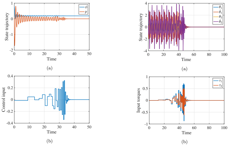
In the paper's simulation examples, the method completes the task even when global Lipschitz continuity or full row rank of g0 fails, and it outperforms linear state feedback in the compared case.

Reading between the lines

Editorial extensions of the paper, not claims the author makes directly.

Beyond the paper's proof, the key differential inequality (21) is asserted to hold from t=0 with Q1(0)=0, but at t=0 the left side is the initial distance to the target, which is positive unless x0 equals x_tg. A corrected argument would need to start the bound from that positive offset; the simulations may still be recoverable, but the theorem as written does not cover them.
The same shrinking-interval construction with a geometric partition, t_n = t_f (1 - a^{-n}), would give finite-horizon arrival and bounded input energy instead of the harmonic schedule's infinite total energy; testing whether the error-bound argument carries over is a direct next step.
For systems with more states than inputs, where g0 is not full row rank, the paper leaves the steady-state error unquantified after the first interval; making that residual explicit would determine when the method is practically useful beyond Assumption 1.
Replacing g0 by g evaluated at the target or at an equilibrium might improve the approximation when drift is large; the paper raises this as a question, and the simulations do not yet resolve it.

Share X Bluesky LinkedIn Reddit HN

Signed reviews

No signed human review yet.

Editorial analysis

A structured set of objections, weighed in public.

Desk editor's note, referee report, and a circularity audit.

Desk Editor's Note

read the letter

Quick take: the paper has a genuinely simple controller idea and honest simulations, but the central convergence theorem is not proven. Equation (21) is false at t=0 unless x0 = xtg, and the same error repeats at every interval boundary. The reader's analysis is right, and the stress-test note is accurate.

What's new: using g(x0) as a driftless model, re-solving a pseudoinverse constant input over harmonic-length intervals is a clean combination. The controller needs almost no model, and the examples (ADMIRE, van der Pol, wing rock, two-link arm) show real behavior. The code is available. The paper is clearly written and the literature is relevant. The self-citation [32] supplies a standard minimum-norm fact; that's fine.

The problem: the proof of Theorem 1. In deriving (21), the constant term ||xtg - x0|| is dropped. Correct combination of (19) and (20) gives dot Q1 <= (||f(x0)|| + DS||xtg-x0||)t + DS Q1 + ||xtg-x0||, not c t + DS Q1. At t=0 the LHS is ||xtg-x0|| and the RHS is 0. The same flaw appears in (32). With the constant term retained, Gronwall yields a bound whose limit over shrinking intervals is the previous error, not zero, so Lemma 1 and Corollary 1 don't follow. The stress-test's scalar example is outside the theorem's assumptions (condition (14) fails because the input constraint isn't satisfied), but that does not rescue the proof: the differential inequality is false under the theorem's own conditions when x0 != xtg.

The simulation section is good supporting material, but simulations cannot patch a false inequality. The method might still work under the restrictive conditions (small drift relative to input authority), but the proof as written doesn't show it, and I'm not convinced the claimed monotone bound holds generally.

Bottom line: reject the paper in its current form. The idea is worth a referee's attention, and a careful author could potentially repair or reframe the proof, but as submitted the central guarantee is unsupported. Would I cite it? No. Bring to reading group? Maybe, as a case study in why the constant term matters in Gronwall arguments.

Referee Report

3 major / 5 minor

Summary. The paper proposes a controller for constrained nonlinear systems (Problem 1) using a sequence of piecewise-constant inputs derived from the linear driftless approximation xdot = g(x0)u. The time horizon is partitioned into intervals of length t*/n, and at each interval the control is the minimum-energy input for the driftless model. The authors claim a monotone bound on the endpoint error, conditions guaranteeing ||u||_infinity <= 1, and convergence to any neighborhood of the target. Section 5 reports simulations on ADMIRE, van der Pol, wing rock, and a two-link robot, with code available.

Significance. The idea is simple and computationally attractive: it uses only g(x0), ignores the drift f, and produces explicitly constructed piecewise-constant inputs. If the theorem were valid, the explicit bound (15) and the input-constraint condition (14) would be a useful contribution. The paper also provides reproducible code and openly discusses assumption violations. However, the main proof is invalid at two load-bearing points, Eqs. (21) and (32), so the central convergence guarantee is not established. The paper cannot be accepted without a substantially different proof.

major comments (3)

[Theorem 1, Eq. (21)] At t=0, inequality (21) reads 0 <= ||xtg - x0||_infinity, which is false unless x0 = xtg; by continuity it fails for small positive t. The correct derivation from (19) and (20) gives \dot Q1(t) <= ||xtg - x0|| + t(||f(x0)|| + D_S ||xtg - x0||) + D_S Q1(t). The constant ||xtg - x0|| cannot be absorbed into c t because c includes (D_S+1)||xtg - x0|| but is multiplied by t. Consequently the Gronwall step leading to (24), and hence the bound (15) for n=1, do not follow.
[Theorem 1, Eq. (32)] The same omission occurs in the induction step: at t = t_k, the right-hand side of (32) is zero while the left-hand side is ||xtg - x_k||, which is not zero in general. Thus the induction step from v_k to v_{k+1} is invalid, and the claim that v_{n+1} <= n/(n+1) v_n applies to the actual error is unsupported. Corollary 1, including the endpoint guarantee and the inter-sample bound, relies on this step.
[Lemma 1 and corrected recurrence] With the corrected inequality, the endpoint error E_k = ||xtg - x_k|| would obey approximately E_{k+1} <= E_k e^{D_S Delta t_{k+1}} + A(e^{D_S Delta t_{k+1}} - 1)/D_S, whose limit as Delta t -> 0 is E_k, not zero. Hence the monotone 1/n contraction asserted in Lemma 1 cannot be concluded from the authors' Gronwall estimate; the argument requires a mechanism that forces E_k itself to decrease, which is absent. The central claim of convergence to the target is therefore not established.

minor comments (5)

[Theorem 1, Part 1] The sentence fragment 'The left-hand side Clearly,' is incomplete; it should read 'Clearly, ||u1(t)||_infinity <= 1 ...'.
[Lemma 1] The definition v_n = c/D_S (e^{Delta t_n D_S} - 1) divides by D_S; the case D_S = 0 should be handled separately or excluded.
[Eq. (14)] The symbol t is overloaded: it is both a variable and the upper bound of the interval for t*. Use a different symbol, e.g., t_max, for the solution of the transcendental equation.
[Corollary 1] In part (ii), t is used for a generic time while t* is the design parameter; this is confusing because t also appears in Eq. (14). Rename one of them.
[Abstract and Section 5.3] The abstract says the method completes the task even when assumptions are violated, but Example 5.3 explicitly reports a non-zero steady-state error. Suggest softening to 'bounded error' or 'satisfactory performance in some cases'.

Circularity Check

0 steps flagged · score 0.0 of 10

No significant circularity: the derivation is self-contained, and the sole self-citation is non-load-bearing.

full rationale

The paper's central claim is Corollary 1, which follows from Theorem 1. The control law (10) is constructed from the pseudoinverse of g0 and the current state, and the error bound (15) is derived from the assumed Lipschitz conditions and a Gronwall-type inequality. No step of this derivation defines the conclusion in terms of itself, and no fitted parameter is relabeled as a prediction. The only same-author citation in the derivation chain is [32], invoked for the minimum-energy property of u1 in (7): “Indeed, it can be shown [32] that (7) is the control input with minimum energy that achieves x(t*)=xtg in (5).” That self-citation is not load-bearing: the subsequent proof uses only the explicit formula (7) and the identity g0 ∫ u1 dt = xtg - x0, not the optimality property. The cited property is also a standard, verifiable pseudoinverse fact, so it does not make the argument circular. The transcendental-equation condition in Lemma 2 and Theorem 1 is cited to [6], not to the authors' own work. The simulations in Section 5 are illustrative and are not used to fit the theoretical bound. There is an apparent mathematical error in the proof of the differential inequality (21) and its analogue (32), as the constant term ‖xtg - x0‖ appears to have been dropped in passing from (19)–(20) to (21); however, an erroneous inequality is a correctness defect, not circular reasoning. For circularity purposes, the derivation chain is self-contained and receives score 0.

Assumptions & free parameters 1 free parameters · 5 assumptions · 0 invented entities

No new physical entities are introduced. The free parameter t* is a design choice. The central claim rests on the global Lipschitz and full-row-rank assumptions and on an asserted differential inequality that is false at t=0.

free parameters (1)

t* (time-horizon design parameter) = 10 (Ex.1), 7 (Ex.2), 9 (Ex.3), 12 (Ex.4)
Chosen by hand as a tuning parameter (Remark 1); the theorem requires it to satisfy (14), but the examples do not verify this.

assumptions (5)

domain assumption f and g are globally Lipschitz with constants D_f and D_g in the infinity norm (Eqs. 2-3)
Used to bound the drift effect in (19), (21), and the induction in Theorem 1.
domain assumption g0 = g(x0) has full row rank N (Assumption 1)
Needed so g0 g0^dagger = I and the constant input (7) exactly reaches the target in the driftless approximation.
ad hoc to paper The differential inequality dot Q1(t) <= c t + D_S Q1(t) (Eq. 21)
Asserted in the proof of Theorem 1 and false at t=0 and nearby, so the Gronwall-based bound (15) is unsupported.
domain assumption The parameter c1 := 2 c ||g0^dagger||_infinity < 1 and t* lies in the interval (14)
The theorem's premise, not established for any particular system; examples choose t* outside this interval.
standard math Gronwall's inequality and the first fundamental theorem of calculus
Standard tools used to convert the differential inequality into the exponential bound.

how reviews work

0 comments

Cite this review

Pith. "Pith review of Ignore Drift, Embrace Simplicity: Constrained Nonlinear Control through Driftless Approximation." pith.science (2026). https://pith.science/paper/SQBVJ5U3

@misc{pith2026250906188,
  author       = {Pith},
  title        = {Pith review of: Ignore Drift, Embrace Simplicity: Constrained Nonlinear Control through Driftless Approximation},
  year         = {2026},
  howpublished = {\url{https://pith.science/paper/SQBVJ5U3}},
  note         = {Machine review of arXiv:2509.06188}
}

read the original abstract

We present a novel technique to drive a nonlinear system to reach a target state under input constraints. The proposed controller consists only of piecewise constant inputs, generated from a simple linear driftless approximation to the original nonlinear system. First, we construct this approximation using only the effect of the control input at the initial state. Next, we partition the time horizon into successively shorter intervals and show that optimal controllers for the linear driftless system result in a bounded error from a specified target state in the nonlinear system. We also derive conditions under which the input constraint is guaranteed to be satisfied. On applying the optimal control inputs, we show that the error monotonically converges to zero as the intervals become successively shorter, thus achieving arbitrary closeness to the target state with time. Using simulation examples on classical nonlinear systems, we illustrate how the presented technique is used to reach a target state while still satisfying input constraints. In particular, we show that our method completes the task even when assumptions of the underlying theory are violated.

Figures

Figures reproduced from arXiv: 2509.06188 by the authors.

**Figure 2.** A simple illustration of convergence behavior from [PITH_FULL_IMAGE:figures/full_fig_p006_2.png] view at source ↗

**Figure 3.** Control of the ADMIRE fighter jet model subjected [PITH_FULL_IMAGE:figures/full_fig_p007_3.png] view at source ↗

Figures from the paper (2 more)

**Figure 4.** Figure 4: Comparing the performance of the proposed method [PITH_FULL_IMAGE:figures/full_fig_p008_4.png]

**Figure 6.** Figure 6: Control of wing rock motion. (a) State trajectories, [PITH_FULL_IMAGE:figures/full_fig_p009_6.png]

Discussion (0). Continue with ORCID to comment.

Forward citations

Cited by 1 Pith paper

Reviewed papers in the Pith corpus that reference this work. Sorted by Pith novelty score. Full citation record

Preferential orientation of slender elastic floaters in gravity waves
physics.flu-dyn 2026-04 unverdicted novelty 6.0 of 10

Wave-induced mean yaw moments drive slender elastic floaters to preferred orientations, with a simple soft/short/heavy vs stiff/long/light criterion for lengths below half a wavelength.

Reference graph

Works this paper leans on

39 extracted references · 38 canonical work pages · cited by 1 Pith paper

[32]

Padmanabhan and M

R. Padmanabhan and M. Ornik. Energetic resilience of linear driftless systems. In11th IF AC Symposium on Robust Control Design, Porto, Portugal, July 2025

work page 2025
[1]

T. M. Apostol.Calculus: Volume 1. John Wiley & Sons, Inc., Hoboken, NJ, USA, 2nd edition, 1967

work page 1967
[2]

Bouvier and M

J.-B. Bouvier and M. Ornik. Designing resilient linear systems.IEEE Transactions on Automatic Control, 67(9):4832–4837, Sep. 2022

work page 2022
[3]

Canudas de Wit and O

C. Canudas de Wit and O. J. Sørdalen. Examples of piecewise smooth stabilization of driftless NL systems with less inputs than states. In2nd IF AC Symposium on Nonlinear Control Systems Design, pages 57–61, Bordeaux, France, June 1992

work page 1992
[4]

Diaz and C

G. Diaz and C. F. M. Coimbra. Nonlinear dynamics and control of a variable order oscillator with application to the van der Pol equation.Nonlinear Dynamics, 56:145–157, April 2009

work page 2009
[5]

Farsi, Y

M. Farsi, Y. Li, Y. Yuan, and J. Liu. A piecewise learning framework for control of unknown nonlinear systems with stability guarantees. In4th Annual Learning for Dynamics and Control Conference, pages 830–843, Palo Alto, CA, USA, June 2022

work page 2022
[6]

T. G. Feeman and O. Marrero. Intersections of tangent lines of exponential functions.The College Mathematics Journal, 36(3):205–208, 2005

work page 2005
[7]

Forssell and U

L. Forssell and U. Nilsson. ADMIRE The aero-data model in a research environment version 4.0, model description. Technical Report FOI-R–1624–SE, FOI – Swedish Defence Research Agency, December 2005

2005

Show all 39 references

[8]

Godhavn, A

J.-M. Godhavn, A. Balluchi, L. Crawford, and S. Sastry. Path planning for nonholonomic systems with drift. In1997 American Control Conference, pages 532–536, Albuquerque, NM, USA, June 1997

1997
[9]

Gromov and F

D. Gromov and F. Casta˜ nos. Control of driftless systems using piecewise constant inputs. In2018 SICE International Symposium on Control Systems, pages 226–231, Tokyo, Japan, March 2018

2018
[10]

Gr¨ une and J

L. Gr¨ une and J. Pannek.Nonlinear Model Predictive Control: Theory and Algorithms. Communcations and Control Engineering. Springer Cham, Cham, Switzerland, 2nd edition, 2018

2018
[11]

J. P. Hespanha.Linear Systems Theory. Princeton University Press, Princeton, NJ, USA, 2nd edition, 2018

2018
[12]

second method

R. E. Kalman and J. E. Bertram. Control system analysis and design via the “second method” of Lyapunov: I—Continuous- time systems.Journal of Basic Engineering, 82(2):371–393, June 1960

1960
[13]

H. K. Khalil.Nonlinear Systems. Prentice Hall, Upper Saddle River, NJ, USA, 3rd edition, 2002

2002
[14]

Leomanni, G

M. Leomanni, G. Costante, and F. Ferrante. Time- optimal control of a multidimensional integrator chain with applications.IEEE Control Systems Letters, 6:2371–2376, February 2022

2022
[15]

Liberzon.Calculus of Variations and Optimal Control Theory: A Concise Introduction

D. Liberzon.Calculus of Variations and Optimal Control Theory: A Concise Introduction. Princeton University Press, Princeton, NJ, USA, 2012

2012
[16]

Y.-J Liu, W. Zhao, L. Liu, D. Li, S. Tong, and C. L. Philip Chen. Adaptive neural network control for a class of nonlinear systems with function constraints on states.IEEE Transactions on Neural Networks and Learning Systems, 34(6):2732–2741, June 2023

2023
[17]

Luo and P

J. Luo and P. Tsiotras. Exponentially convergent control laws for nonholonomic systems in power form.Systems & Control Letters, 35(2):87–95, September 1998

1998
[18]

Magni and R

L. Magni and R. Scattolini. Model predictive control of continuous-time nonlinear systems with piecewise constant control.IEEE Transactions on Automatic Control, 49(6):900–906, June 2004

2004
[19]

Y. Meng, T. Shafa, J. Wei, and M. Ornik. Online learning and control synthesis for reachable paths of unknown nonlinear systems, 2024. https://arxiv.org/abs/2403.03413

2024 arXiv
[20]

Mesbahi and M

M. Mesbahi and M. Egerstedt.Graph Theoretic Methods in Multiagent Networks. Princeton University Press, Princeton, NJ, USA, 2010

2010
[21]

M. M. Monahemi and M. Krstic. Control of wing rock motion using adaptive feedback linearization.Journal of Guidance, Control and Dynamics, 19(4):905–912, July 1996

1996
[22]

Morin and C

P. Morin and C. Samson. Exponential stabilization of nonlinear driftless systems with robustness to unmodeled dynamics.ESAIM: Control, Optimisation and Calculus of Variations, 4:1–35, April 1999

1999
[23]

R. T. M’Closkey.Exponential stabilization of driftless nonlinear control systems. PhD thesis, California Institute of Technology, 1995

1995
[24]

C. P. Niculescu and L.-E Persson.Convex Functions and Their Applications: A Contemporary Approach. Springer, New York, NY, USA, 2006

2006
[25]

Nijmeijer and A

H. Nijmeijer and A. van der Schaft.Nonlinear Dynamical Control Systems. Springer-Verlag, New York, NY, USA, 1990

1990
[26]

O. J. Oaks and G. Cook. Piecewise linear control of nonlinear systems.IEEE Transactions on Industrial Electronics and Control Instrumentation, IECI-23(1):56–63, February 1976

1976
[27]

Ohtake, K

H. Ohtake, K. Tanaka, and H.O. Wang. Piecewise nonlinear control. In42nd IEEE Conference on Decision and Control, pages 4735–4740, Maui, HI, USA, December 2003. 11

2003
[28]

Oshima, S

T. Oshima, S. Kawai, and T. Nguyen-Van. A discrete-time linearization feedback control for the Van der Pol oscillator. In61st Annual Conference of the Society of Instrument and Control Engineers, pages 574–579, Kumamoto, Japan, September 2022

2022
[29]

¨Ozkan, M

L. ¨Ozkan, M. V. Kothare, and C. Georgakis. Model predictive control of nonlinear systems using piecewise linear models. Computers & Chemical Engineering, 24(2-7):793–799, July 2000

2000
[30]

B. G. Pachpatte.Inequalities for Differential and Integral Equations. Academic Press Limited, London, United Kingdom, 1998

1998
[31]

Padmanabhan and M

R. Padmanabhan and M. Ornik. Approximate energetic resilience of nonlinear systems under partial loss of control authority, 2025. https://arxiv.org/abs/2502.07603

2025
[33]

R. Penrose. On best approximate solutions of linear matrix equations.Mathematical Proceedings of the Cambridge Philosophical Society, 52(1):17–19, January 1956

1956
[34]

Sarangapani.Neural Network Control of Nonlinear Discrete-Time Systems

J. Sarangapani.Neural Network Control of Nonlinear Discrete-Time Systems. Taylor & Francis Group, Boca Raton, FL, USA, 2006

2006
[35]

Sinha, F

M. Sinha, F. D¨ orfler, B. Johnson, and S. Dhople. Stabilizing phase-balanced or phase-synchronized trajectories of Van der Pol oscillators in uniform electrical networks. In56th Annual Allerton Conference on Communication, Control, and Computing, pages 335–340, Monticello, IL...

2018
[36]

E. D. Sontag. Nonlinear regulation: The piecewise linear approach.IEEE Transactions on Automatic Control, 26(2):346–358, April 1981

1981
[37]

V. I. Utkin.Sliding Modes in Control and Optimization. Communications and Control Engineering. Springer-Verlag, Heidelberg, Germany, 1992

1992
[38]

S. T. Venkataraman and S. Gulati. Control of nonlinear systems using terminal sliding modes. In1992 American Control Conference, pages 891–893, Chicago, IL, USA, June 1992

1992
[39]

Q. Wang, W. Wang, and S. Suzuki. UA V trajectory tracking under wind disturbance based on novel antidisturbance sliding mode control.Aerospace Science and Technology, 149, June 2024. 12

2024

Pith tools

Reviewed August 4, 2026 · model on record in the stance chip above.

[1] [32]

Padmanabhan and M

R. Padmanabhan and M. Ornik. Energetic resilience of linear driftless systems. In11th IF AC Symposium on Robust Control Design, Porto, Portugal, July 2025

work page 2025

[2] [1]

T. M. Apostol.Calculus: Volume 1. John Wiley & Sons, Inc., Hoboken, NJ, USA, 2nd edition, 1967

work page 1967

[3] [2]

Bouvier and M

J.-B. Bouvier and M. Ornik. Designing resilient linear systems.IEEE Transactions on Automatic Control, 67(9):4832–4837, Sep. 2022

work page 2022

[4] [3]

Canudas de Wit and O

C. Canudas de Wit and O. J. Sørdalen. Examples of piecewise smooth stabilization of driftless NL systems with less inputs than states. In2nd IF AC Symposium on Nonlinear Control Systems Design, pages 57–61, Bordeaux, France, June 1992

work page 1992

[5] [4]

Diaz and C

G. Diaz and C. F. M. Coimbra. Nonlinear dynamics and control of a variable order oscillator with application to the van der Pol equation.Nonlinear Dynamics, 56:145–157, April 2009

work page 2009

[6] [5]

Farsi, Y

M. Farsi, Y. Li, Y. Yuan, and J. Liu. A piecewise learning framework for control of unknown nonlinear systems with stability guarantees. In4th Annual Learning for Dynamics and Control Conference, pages 830–843, Palo Alto, CA, USA, June 2022

work page 2022

[7] [6]

T. G. Feeman and O. Marrero. Intersections of tangent lines of exponential functions.The College Mathematics Journal, 36(3):205–208, 2005

work page 2005

[8] [7]

Forssell and U

L. Forssell and U. Nilsson. ADMIRE The aero-data model in a research environment version 4.0, model description. Technical Report FOI-R–1624–SE, FOI – Swedish Defence Research Agency, December 2005

2005