Sequential Least-Squares Estimators with Fast Randomized Sketching for Linear Statistical Models

Dong-Yue Xie; Guan-Yu Chen; Xi Yang

REVIEW 3 major objections 4 minor 25 references

Sequential Least-Squares Estimators with Fast Randomized Sketching for Linear Statistical Models

T0 review · 3 major / 4 minor · reviewed 2026-08-04 · deepseek-v4-flash

Challenge this review Re-run · record.json Download PDF Read on arXiv ↗

Pith's one-line read This paper claims a warm-started ladder of sketched least-squares subproblems, finished by a few full-scale iterations, reproduces the exact OLS prediction error up to a vanishing term at cost dominated by one fast transform pass.

desk verdict The sequential sketch-size idea is worth a look, but the main OLS-accuracy theorem is not proved as stated and needs a serious repair before I'd trust the paper's headline. read the letter →

arxiv 2509.06856 v2 pith:YPLW23N4 submitted 2025-09-08 stat.ML cs.LGcs.NAmath.NA

Guan-Yu Chen , Dong-Yue Xie , Xi Yang This is my paper · ORCID

classification stat.MLcs.LGcs.NAmath.NA MSC 62J0565F1068W20

keywords linearregressionrandomizedsketchingSketch-and-SolveIterativeHessianSketchSRHTmomentumpredictionerrorlarge-scaleleastsquares

verification ladder T0 review T1 audit T2 compute T3 formal

The pith

A machine-rendered reading of the paper's core claim, the machinery that carries it, and where it could break.

The reading

The paper proposes SLSE-FRS, a framework for large-scale linear regression that combines two previously separate randomized strategies: Sketch-and-Solve and Iterative Sketching. Instead of relying on a single sketched fit, whose precision is capped by the sketch size, or iterating directly on the full data, SLSE-FRS solves a sequence of sketched least-squares subproblems with doubling sketch sizes, each warm-started from the previous solution, and then runs a few full-scale momentum iterations. The central theorem states that, with high probability, the final estimator's expected prediction error equals that of the exact ordinary least-squares estimator up to a term that vanishes as the inner iteration counts grow, while the total cost is dominated by a single Nd log N Hadamard pass over the data. The numerical experiments show the method reaching OLS-level error in less wall-clock time than the preconditioned conjugate gradient and iterative double sketching baselines. This matters because it suggests that OLS-quality estimates are affordable in regimes where the direct O(N d²) solve is prohibitive.

What carries the argument

The engine is a two-stage inner-outer iteration. The outer stage constructs K sketched least-squares problems from one SRHT-transformed copy of the data: (S_i X, S_i Y) is extracted by sampling rows of the full transformed data, so building all subproblems costs one Nd log N Hadamard pass. The inner stage runs momentum iterative Hessian sketch (M-IHS) with a fixed randomized preconditioner Ĥ and heavy-ball parameters η = 53/36 − √(17/3), µ = (1 − η)²; the two-step recurrence is decomposed into a 2×2 block iteration matrix whose spectral radius, via the Gelfand formula, is √η < 1/3, giving the (1/3)^{a_i} contraction per subproblem. The precision ladder itself is set by the asymptotic relativ

What would settle it

Estimate, on the paper's own test designs (e.g., N = 2²⁰, d = 2⁶, κ = 10⁴), the ratio E‖X(β̃_i − β)‖ / E‖X(β̂ − β)‖ at each sketch size m_i and check the variance inequality Var(‖X(β̃_i − β)‖) ≥ Var(√((N−d)/(m_i−d)) ‖X(β̂ − β)‖) stated in Remark A.7. If the inequality fails at moderate N, the [1 + o(1)] OLS-equivalence conclusion of Theorem 4.2 lacks its stated support; one could then test whether running SLSE-FRS with the recommended a_i = 2 or 3 still drives the prediction error down to the σ-level.

Watch

Extended reading notes

Core claim

On its own terms, the paper's discovery is that the suboptimality of Sketch-and-Solve — the precision ceiling imposed by a fixed sketch size — can be exploited as a schedule rather than treated as a limitation. By choosing sketch sizes that double (m_{i+1} = 2m_i), using the δ_i-level error of each exact sketched estimator as the stopping target for a momentum iterative-Hessian-sketch solver, and letting errors decay through the (1/3)^{a_i} contraction of a heavy-ball iteration matrix, the final output satisfies E‖X(β_T − β)‖ ≤ (1/3)^T E‖X(β_0 − β)‖ + [1 + o(1)] E‖X(β̂ − β)‖. In words: the algorithm attains the same expected prediction error as the exact ordinary least-squares estimator, up

Load-bearing premise

Theorem 4.2's proof needs E‖X(β̃_i − β)‖ ≤ √((N−d)/(m_i−d)) E‖X(β̂ − β)‖, which combines an infinite-sample spectral-limit result with an unproved variance ordering of the two prediction errors; if that variance ordering fails at finite N, the claimed OLS-matching precision does not follow from the stated assumptions.

Editorial extensions

If this is right

SLSE-FRS reaches OLS-level (σ-level) prediction error with only about 2–3 iterations per sketched subproblem, so per-iteration cost scales with the sketch size m_i rather than the sample size N.
The total complexity is dominated by initialization at Nd log₂ N; if log N is treated as constant the pipeline is O(Nd), and replacing SRHT by CountSketch would make it rigorously O(Nd) once the corresponding embedding theorems are proved.
Because each subproblem only needs to reach the sketched estimator's own precision δ_i, any current or future iterative least-squares solver can be plugged into the framework, provided a δ_i-level stopping criterion can be established.
The worst-case convergence rate of 1/3 is tied to the chosen heavy-ball parameters, and the paper notes that alternative parameter settings can yield a sharper rate.
The sketch-size sequence can be tuned by hand, as in the tuning experiment that skips large intermediate sizes, to cut computing time further, though an automatic tuning strategy remains open.

Reading between the lines

Editorial extensions of the paper, not claims the author makes directly.

The 'precision ladder' design principle generalizes beyond linear least squares: whenever an iterative solver's per-iteration cost is proportional to the data it sees, running it to only the precision of the current sketch before enlarging the sketch is a near-optimal way to allocate compute; the same pattern could apply to logistic regression or other smooth objectives with sketched Hessians.
The load-bearing variance ordering in Remark A.7 is empirically checkable on the paper's own test designs; a reader who computes Var(‖Xβ̃_i − Xβ‖) against Var(√((N−d)/(m_i−d))‖Xβ̂ − Xβ‖) at finite N would learn whether the OLS-matching guarantee is actually active in the experiments.
The theory assumes the empirical spectral distribution of X approaches a compact-support limit; designs with heavy-tailed or otherwise non-limiting spectra might degrade the OLS-equivalence guarantee even when the iteration counts match the recommended a_i = 2 or 3, a testable boundary of the method.
The warm-start structure multiplies errors across subproblems by (1/3)^{a_i} factors rather than adding them, so poor initial guesses are forgotten quickly; this makes the method's success relatively insensitive to β_0, a property the paper does not showcase but that follows from the proof chain.

Share X Bluesky LinkedIn Reddit HN

Editorial analysis

A structured set of objections, weighed in public.

Desk editor's note, referee report, and a circularity audit.

Desk Editor's Note

read the letter

Read it. The genuinely new piece is the sequential construction of sketched LS subproblems with doubling sketch sizes, each solved with a few M-IHS iterations and warm-started from the previous subproblem. That is a sensible multilevel idea, and the experiments showing 2–3x speedups over IDS and PCG are consistent with the claim that it pays off. The paper is honest about the ingredients being prior art (Sketch-and-Solve, M-IHS, nested sketch data from Wang et al.), and the writing is clear.

The soft spot is Theorem 4.2. The claimed OLS-level guarantee is not proven under the assumptions stated in the theorem. The proof goes through Lemma A.8, which uses Remark A.7 to replace E||X(tildeβ_i - β)|| by sqrt((N-d)/(m_i-d)) E||X(hatβ-β)||. That step needs two things that never appear in Theorem 4.2: convergence of the empirical spectral distribution of X (and the limits d/N→γ, m_i/N→ξ), and a variance inequality Var(||Xtildeβ_i−Xβ||) ≥ Var(sqrt((N−d)/(m_i−d)) ||Xhatβ−Xβ||). The variance inequality is doing real work: without it, the squared-norm PE bound from Dobriban–Liu doesn't imply the E-norm inequality; there is a Jensen gap. Neither condition is checked in the experiments. On top of that, Lemma A.6 is an asymptotic statement in N, while the o(1) in (11) is declared as M→∞, and the proof never reconciles those two limits. So as it stands, the main theorem is conditional on assumptions not stated.

A smaller issue: Theorem 4.3's lower bound on a_i relies on the contraction (15), which only holds once a_i exceeds a constant M_i. The theorem doesn't show the recommended a_i is above that threshold; the experiments use a_i=2 or 3 with no indication of where M_i sits. This one is repairable by restating the theorem with the threshold condition.

The paper ships no code or data, so the empirical speedups aren't independently reproducible. That matters less than the proof gap, but it matters.

I think the idea is good and the proof has a specific, likely fixable hole. I would send it to a serious referee, but I would not cite the OLS-level guarantee as it stands. A revised version that proves or removes the variance condition and states the spectral assumptions inside Theorem 4.2 would change my mind.

Referee Report

3 major / 4 minor

Summary. The paper proposes a two-stage randomized algorithm, SLSE-FRS, for large-scale linear least squares. In the first stage it sequentially solves K sketched least-squares subproblems with doubling sketch sizes, using M-IHS iterations to approximately solve each subproblem; the second stage applies M-IHS to the full problem starting from the accumulated estimator. The main theoretical claims are: (i) each subproblem converges to its exact sketched LS estimator at rate 1/3 (Theorem 4.1); (ii) the final estimator attains the OLS prediction error up to a vanishing term (Theorem 4.2); (iii) a lower bound on the number of inner iterations (Theorem 4.3); and (iv) total complexity dominated by Nd log N (Theorem 4.4). Numerical experiments compare SLSE-FRS with IDS, PCG, and M-IHS on synthetic data.

Significance. If Theorem 4.2 were proved under only the assumptions stated in Section 4, SLSE-FRS would be a notable contribution: it would be the first algorithm to combine Sketch-and-Solve and Iterative Sketching in this sequential way and would reach OLS precision in near-linear time, with a clear complexity advantage over IDS and PCG. The paper also gives a careful FLOP accounting and a flexible framework. However, the advertised OLS-precision guarantee is not established by the proof as written: it depends on asymptotic spectral-distribution assumptions and on an unstated variance inequality in Remark A.7, and the finite-N/asymptotic limit exchange is not handled. These issues are load-bearing for the main claim, so the theoretical contribution cannot currently be taken at face value.

major comments (3)

[Theorem 4.2 (Section 4) and Appendix A.3, Lemma A.8 / Remark A.7] Central bound (11) in Theorem 4.2 is not proved under the theorem's stated assumptions. The proof of Lemma A.8 uses Lemma A.6 to write E||X(tildeβ_i−Xβ)||^2 ≤ ((N−d)/(m_i−d)) E||X(hatβ−Xβ)||^2, and then uses the variance condition Var(||Xtildeβ_i−Xβ||) ≥ Var(sqrt((N−d)/(m_i−d))||Xhatβ−Xβ||) from Remark A.7 to convert this into the E-norm ratio. Neither the variance condition nor the asymptotic spectral-distribution conditions (d/N→γ, m_i/N→ξ∈(γ,1)) appear in Theorem 4.2 or in Lemma A.8, and the experiments do not check them. Without the variance condition, the E-norm bound does not follow from the squared-norm PE bound; a Jensen gap remains. Thus the [1+o(1)]E||X(hatβ−β)|| term in (11) is unsupported for the general designs allowed by the theorem statement.
[Appendix A.3, Lemma A.6 and Lemma A.8; Theorem 4.2] There is an unreconciled double limit. Lemma A.6 is an asymptotic statement as N→∞ with d/N→γ and m_i/N→ξ. Theorem 4.2 is stated for fixed N, m_1 powers of two, and its o(1) in (11) is declared to be as M→∞. The proof applies the asymptotic PE bound to the finite-N problem and provides no finite-N remainder. The o(1) in Eq. (20) is as M†→∞, not as N→∞. A rigorous proof needs either explicit non-asymptotic error bounds for Lemma A.6 or a restatement of Theorem 4.2 as a double-limit result with controlled error terms.
[Theorem 4.3 and Appendix A.5] The lower bound a_i ≥ log_3(((1+ω)r(i−1,i)+1)/ω) relies on two ingredients that are not stated as hypotheses: the asymptotic contraction (15), which only holds for a_i > M_i with the existential constant from Theorem 4.1, and the relation E||X(tildeβ_{i−1}−Xβ)|| ≤ r(i−1,i) E||X(tildeβ_i−Xβ)||, which again uses Lemma A.6/Remark A.7. The theorem statement gives no regime in which either ingredient is valid. Consequently, the bound is not a standalone finite-iteration guarantee. Please restate Theorem 4.3 with all hypotheses, including the validity range of (15) and (24).

minor comments (4)

[Throughout, Eq. (7)-(8) and Theorems 4.1-4.2] The parameter η is written as 53/36 − √17/3. As typeset this is ambiguous: √(17/3) ≈ 2.38 would make η negative. It should be √17/3 = (√17)/3. Please fix the notation.
[Algorithm 1 and Algorithm 2] The input line says Y∈R^d; the response vector is in R^N. This appears to be a typo.
[Section 2, paragraph after Algorithm 1] The sentence 'In Section 1.1, we will introduce an efficient implementation...' should refer to Section 3, where the M-IHS implementation is actually given.
[Theorem 4.4] The termination criterion 'achieves the noise level σ' is not defined in the linear model context. In the model, the noise standard deviation is σ and the OLS prediction error is of order σ√d; the proof sets T=log_3(1/σ), treating σ as a dimensionless relative tolerance. Please clarify the target precision and reconcile the notation.

Circularity Check

0 steps flagged · score 0.0 of 10

No circularity: the main bounds derive from spectral-radius contraction and external asymptotic PE results, not from fitted quantities or self-citations.

full rationale

The derivation chain is not circular. The contraction factor 1/3 in Theorem 4.1 comes from a spectral-radius analysis of the M-IHS iteration matrix L^(i), with the heavy-ball parameter η chosen from a quadratic inequality; no fitted parameter is used. The passage from the sketch-subproblem error δ_i to the OLS error E||X(hatβ−β)|| in Lemma A.8 uses the asymptotic PE formula of Dobriban and Liu (2019) plus a variance inequality stated in Remark A.7. That variance inequality is not proved or verified, so Theorem 4.2 is not established under its stated assumptions; this is a proof gap/correctness risk, not a circular reduction. The iteration-count lower bounds in Theorem 4.3 and complexity claims in Theorem 4.4 likewise reuse external PE asymptotics and standard FLOP counts, and the experiments compare against IDS/PCG/M-IHS rather than fitting a parameter to force the theorem. There is no instance where a quantity is defined in terms of the target, a fitted input is relabeled a prediction, or a load-bearing premise depends on a self-citation. The SRHT embedding theorem is cited from Wang et al. (2022) and the PE asymptotics from Dobriban and Liu (2019), both independent of the present authors, and neither is used to define away the target result.

Assumptions & free parameters 5 free parameters · 7 assumptions · 0 invented entities

The central convergence result depends on external embedding and asymptotic results, plus several conditions stated only in remarks. No new physical or modeled entities are introduced; SLSE-FRS is an algorithmic framework. The most load-bearing unstated item is the variance condition in Remark A.7, which is needed to convert second-moment bounds into the first-moment form used in the theorems.

free parameters (5)

m_1 (initial sketch size) = 8d
Chosen as 8d in all experiments; theory only requires m_1 > r = O(d log d).
Sketch size growth ratio = m_{i+1}/m_i = 2
Chosen for nested row sampling and to have K = log2(N/m1) subproblems.
r (Hessian sketch size) = 6d
Used in all experiments; theory requires r = Ω(d log d).
a_i (inner iteration counts) = 2 or 3
Selected from a single tuning experiment (Section 5.1); then used in all other experiments.
μ, η (momentum and step parameters) = η=53/36−√17/3≈0.0978; μ=(1−η)^2 in experiments
Derived from spectral-radius analysis, but the experimental μ follows Ozaslan et al.; not fitted to data.

assumptions (7)

standard math SRHT is a (1+ε) subspace embedding with m = O(d log d) (Theorem 3.2 from Wang et al. 2022).
Invoked in Lemma A.1 to bound ||U^T S_i^T S_i U - I|| and in the Hessian sketch construction.
domain assumption Asymptotic PE formula from Dobriban and Liu (Lemma A.6): PE(i) tends to (1−γ)/(ξ−γ).
Used in Lemma A.8 and Theorem 4.3 to relate sketched estimator error to OLS error; requires N→∞ with d/N→γ and m_i/N→ξ.
ad hoc to paper Variance condition: Var(||X˜β_i−Xβ||) ≥ Var(√((N−d)/(m_i−d)) ||Xhatβ−Xβ||).
Stated only in Remark A.7 as a basis for the first-moment bound. It is not proven, not stated in the main theorems, and not checked in experiments.
domain assumption Empirical spectral distribution of X converges to a fixed distribution with compact support bounded away from the origin.
Condition for Lemma A.6 from Dobriban and Liu, used in the error analysis.
domain assumption X has full column rank and N is a power of 2.
Stated in the introduction and needed for the explicit OLS formula and the fast Hadamard transform.
standard math Gelfand formula and heavy-ball iteration analysis (Recht 2010).
Used in the proof of Theorem 4.1 to obtain the (1/3)^{a_i} contraction for sufficiently large a_i.
ad hoc to paper Initial-error ratio condition: 1 < E||X(β0−˜β1)||/E||X(˜β1−β)|| < 1+(1+ω)/√2.
Assumed in Theorem 4.4 to bound a_1 and the total cost; no justification is provided.

how reviews work

0 comments

Cite this review

Pith. "Pith review of Sequential Least-Squares Estimators with Fast Randomized Sketching for Linear Statistical Models." pith.science (2026). https://pith.science/paper/YPLW23N4

@misc{pith2026250906856,
  author       = {Pith},
  title        = {Pith review of: Sequential Least-Squares Estimators with Fast Randomized Sketching for Linear Statistical Models},
  year         = {2026},
  howpublished = {\url{https://pith.science/paper/YPLW23N4}},
  note         = {Machine review of arXiv:2509.06856}
}

read the original abstract

We propose a novel randomized framework for the estimation problem of large-scale linear statistical models, namely Sequential Least-Squares Estimators with Fast Randomized Sketching (SLSE-FRS), which integrates Sketch-and-Solve and Iterative-Sketching methods for the first time. By iteratively constructing and solving sketched least-squares (LS) subproblems with increasing sketch sizes to achieve better precisions, SLSE-FRS gradually refines the estimators of the true parameter vector, ultimately producing high-precision estimators. We analyze the convergence properties of SLSE-FRS, and provide its efficient implementation. Numerical experiments show that SLSE-FRS outperforms the state-of-the-art methods, namely the Preconditioned Conjugate Gradient (PCG) method, and the Iterative Double Sketching (IDS) method.

Figures

Figures reproduced from arXiv: 2509.06856 by the authors.

**Figure 1.** The iteration control parameter ai for SLSE-FRS: a2, aK versus ω; computing time versus ai = NoI (the number of iterations of the sketched LS subproblems) for all i. 9 [PITH_FULL_IMAGE:figures/full_fig_p009_1.png] view at source ↗

**Figure 2.** ∆T of SLSE-FRS and ∆ of OLS and iteration paths of SLSE-FRS and IDS. In [PITH_FULL_IMAGE:figures/full_fig_p010_2.png] view at source ↗

**Figure 3.** ∆t versus iterations and actual computing time for SLSE-FRS, IDS and PCG. 0 5 10 15 20 25 30 35 Iteration -10 -5 0 5 10 15 Log error to truth M-IHS SLSE-FRS Target accuracy (a) N = 220, d = 26 1.5 2 2.5 3 3.5 4 Actual Time (seconds) -5 0 5 10 Log error to truth M-IHS SLSE-FRS Target accuracy (b) N = 220, d = 26 [PITH_FULL_IMAGE:figures/full_fig_p011_3.png] view at source ↗

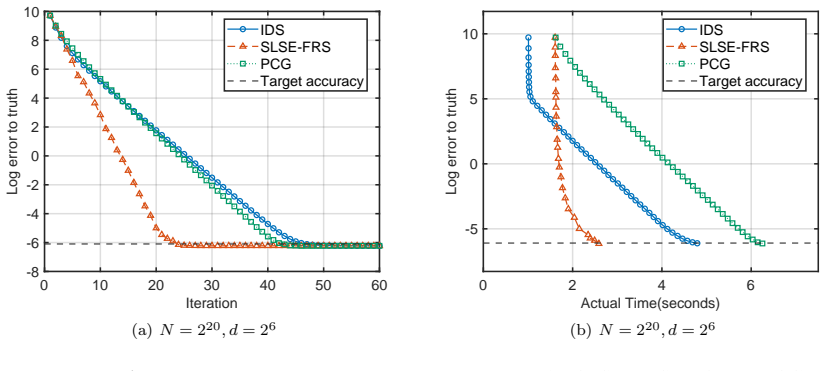
Figures from the paper (4 more)

**Figure 4.** Figure 4: ∆t versus iterations and actual computing time for SLSE-FRS and M-IHS. 0 5 10 15 20 25 30 Iteration -6 -4 -2 0 2 4 6 8 Log error to truth IDS SLSE-FRS Target accuracy (a) N = 220, d = 210 15 20 25 30 35 40 Actual Time (seconds) -6 -4 -2 0 2 4 6 Log error to truth IDS S…

**Figure 5.** Figure 5: ∆t versus iterations and actual computing time for SLSE-FRS and IDS. 11 [PITH_FULL_IMAGE:figures/full_fig_p011_5.png]

**Figure 6.** Figure 6: ∆t versus iterations and actual computing time for SLSE-FRS, SLSE-FRS-tuning, IDS and PCG. 12 [PITH_FULL_IMAGE:figures/full_fig_p012_6.png]

**Figure 7.** Figure 7: ∆t versus iterations and actual computing time for SLSE-FRS-SRHT, SLSE-FRS-CS and IDS. 6 Discussion In this work, we introduced the novel SLSE-FRS framework for large-scale estimation problem of linear statistical models which iteratively constructs and solves sketched…

Discussion (0). Continue with ORCID to comment.

Reference graph

Works this paper leans on

25 extracted references · 21 canonical work pages

[1]

The fast Johnson-Lindenstrauss transform and approximate nearest neighbors

Nir Ailon and Bernard Chazelle. The fast Johnson-Lindenstrauss transform and approximate nearest neighbors. SIAM Journal on Computing, 39 0 (1): 0 302--322, 2009

work page 2009
[2]

Sensitivity analysis in linear regression

Samprit Chatterjee and Ali S Hadi. Sensitivity analysis in linear regression. John Wiley & Sons, 2009

work page 2009
[3]

Low-rank approximation and regression in input sparsity time

Kenneth L Clarkson and David P Woodruff. Low-rank approximation and regression in input sparsity time. Journal of the ACM, 63 0 (6): 0 1--45, 2017

work page 2017
[4]

Recent and upcoming developments in randomized numerical linear algebra for machine learning

Micha Derezi \'n ski and Michael W Mahoney. Recent and upcoming developments in randomized numerical linear algebra for machine learning. In Proceedings of the 30th ACM SIGKDD Conference on Knowledge Discovery and Data Mining, pages 6470--6479, 2024

2024
[5]

Asymptotics for sketching in least squares regression

Edgar Dobriban and Sifan Liu. Asymptotics for sketching in least squares regression. Advances in Neural Information Processing Systems, 32, 2019

work page 2019
[6]

RandNLA : randomized numerical linear algebra

Petros Drineas and Michael W Mahoney. RandNLA : randomized numerical linear algebra. Communications of the ACM, 59 0 (6): 0 80--90, 2016

work page 2016
[7]

Sampling algorithms for _2 regression and applications

Petros Drineas, Michael W Mahoney, and Shan Muthukrishnan. Sampling algorithms for _2 regression and applications. In Proceedings of the Seventeenth Annual ACM-SIAM Symposium on Discrete Algorithm, pages 1127--1136, 2006

work page 2006
[8]

Faster least squares approximation

Petros Drineas, Michael W Mahoney, Shan Muthukrishnan, and Tam \'a s Sarl \'o s. Faster least squares approximation. Numerische mathematik, 117 0 (2): 0 219--249, 2011

work page 2011

Show all 25 references

[9]

Fast and forward stable randomized algorithms for linear least-squares problems

Ethan N Epperly. Fast and forward stable randomized algorithms for linear least-squares problems. SIAM Journal on Matrix Analysis and Applications, 45 0 (4): 0 1782--1804, 2024

2024
[10]

Matrix computations

Gene H Golub and Charles F Van Loan. Matrix computations. JHU Press, 2013

2013
[11]

Approximate nearest neighbors: towards removing the curse of dimensionality

Piotr Indyk and Rajeev Motwani. Approximate nearest neighbors: towards removing the curse of dimensionality. In Proceedings of the Thirtieth Annual ACM Symposium on Theory of Computing, pages 604--613, 1998

1998
[12]

On accuracy of approximation of the spectral radius by the gelfand formula

Victor Kozyakin. On accuracy of approximation of the spectral radius by the gelfand formula. Linear Algebra and its Applications, 431 0 (11): 0 2134--2141, 2009

2009
[13]

Optimal randomized first-order methods for least-squares problems

Jonathan Lacotte and Mert Pilanci. Optimal randomized first-order methods for least-squares problems. In International Conference on Machine Learning, pages 5587--5597, 2020

2020
[14]

Faster least squares optimization

Jonathan Lacotte and Mert Pilanci. Faster least squares optimization. arXiv preprint arXiv:1911.02675, 2021

1911 arXiv
[15]

Adaptive newton sketch: Linear-time optimization with quadratic convergence and effective hessian dimensionality

Jonathan Lacotte, Yifei Wang, and Mert Pilanci. Adaptive newton sketch: Linear-time optimization with quadratic convergence and effective hessian dimensionality. In International Conference on Machine Learning, pages 5926--5936, 2021

2021
[16]

Randomized numerical linear algebra: foundations & algorithms

Per-Gunnar Martinsson and Joel Tropp. Randomized numerical linear algebra: foundations & algorithms. arXiv preprint arXiv:2002.01387, 2020

2002 arXiv
[17]

Hessian averaging in stochastic Newton methods achieves superlinear convergence

Sen Na, Micha Derezi \'n ski, and Michael W Mahoney. Hessian averaging in stochastic Newton methods achieves superlinear convergence. Mathematical Programming, 201 0 (1): 0 473--520, 2023

2023
[18]

Iterative Hessian sketch with momentum

Ibrahim Kurban Ozaslan, Mert Pilanci, and Orhan Arikan. Iterative Hessian sketch with momentum. In IEEE International Conference on Acoustics, Speech and Signal Processing, pages 7470--7474, 2019

2019
[19]

Iterative Hessian sketch: Fast and accurate solution approximation for constrained least-squares

Mert Pilanci and Martin J Wainwright. Iterative Hessian sketch: Fast and accurate solution approximation for constrained least-squares. Journal of Machine Learning Research, 17 0 (53): 0 1--38, 2016

2016
[20]

Newton sketch: A near linear-time optimization algorithm with linear-quadratic convergence

Mert Pilanci and Martin J Wainwright. Newton sketch: A near linear-time optimization algorithm with linear-quadratic convergence. SIAM Journal on Optimization, 27 0 (1): 0 205--245, 2017

2017
[21]

CS726 - Lyapunov analysis and the heavy ball method

Benjamin Recht. CS726 - Lyapunov analysis and the heavy ball method. Department of Computer Sciences, University of Wisconsin--Madison, 2010

2010
[22]

Improved approximation algorithms for large matrices via random projections

Tamas Sarlos. Improved approximation algorithms for large matrices via random projections. In 47th Annual IEEE Symposium on Foundations of Computer Science, pages 143--152, 2006

2006
[23]

Gradient projection iterative sketch for large-scale constrained least-squares

Junqi Tang, Mohammad Golbabaee, and Mike E Davies. Gradient projection iterative sketch for large-scale constrained least-squares. In International Conference on Machine Learning, pages 3377--3386, 2017

2017
[24]

Iterative double sketching for faster least-squares optimization

Rui Wang, Yanyan Ouyang, and Wangli Xu. Iterative double sketching for faster least-squares optimization. In International Conference on Machine Learning, pages 22935--22963, 2022

2022
[25]

Sketching as a tool for numerical linear algebra

David P Woodruff et al. Sketching as a tool for numerical linear algebra. Foundations and Trends in Theoretical Computer Science , 10 0 (1--2): 0 1--157, 2014

2014

Pith tools

Reviewed August 4, 2026 · model on record in the stance chip above.

[1] [1]

The fast Johnson-Lindenstrauss transform and approximate nearest neighbors

Nir Ailon and Bernard Chazelle. The fast Johnson-Lindenstrauss transform and approximate nearest neighbors. SIAM Journal on Computing, 39 0 (1): 0 302--322, 2009

work page 2009

[2] [2]

Sensitivity analysis in linear regression

Samprit Chatterjee and Ali S Hadi. Sensitivity analysis in linear regression. John Wiley & Sons, 2009

work page 2009

[3] [3]

Low-rank approximation and regression in input sparsity time

Kenneth L Clarkson and David P Woodruff. Low-rank approximation and regression in input sparsity time. Journal of the ACM, 63 0 (6): 0 1--45, 2017

work page 2017

[4] [4]

Recent and upcoming developments in randomized numerical linear algebra for machine learning

Micha Derezi \'n ski and Michael W Mahoney. Recent and upcoming developments in randomized numerical linear algebra for machine learning. In Proceedings of the 30th ACM SIGKDD Conference on Knowledge Discovery and Data Mining, pages 6470--6479, 2024

2024

[5] [5]

Asymptotics for sketching in least squares regression

Edgar Dobriban and Sifan Liu. Asymptotics for sketching in least squares regression. Advances in Neural Information Processing Systems, 32, 2019

work page 2019

[6] [6]

RandNLA : randomized numerical linear algebra

Petros Drineas and Michael W Mahoney. RandNLA : randomized numerical linear algebra. Communications of the ACM, 59 0 (6): 0 80--90, 2016

work page 2016

[7] [7]

Sampling algorithms for _2 regression and applications

Petros Drineas, Michael W Mahoney, and Shan Muthukrishnan. Sampling algorithms for _2 regression and applications. In Proceedings of the Seventeenth Annual ACM-SIAM Symposium on Discrete Algorithm, pages 1127--1136, 2006

work page 2006

[8] [8]

Faster least squares approximation

Petros Drineas, Michael W Mahoney, Shan Muthukrishnan, and Tam \'a s Sarl \'o s. Faster least squares approximation. Numerische mathematik, 117 0 (2): 0 219--249, 2011

work page 2011