REVIEW 4 major objections 5 minor 62 references
Quantum Filtering and Stabilization of Dissipative Quantum Systems via Augmented Neural Ordinary Differential Equations
T0 review · 4 major / 5 minor · reviewed 2026-08-04 · deepseek-v4-flash
Pith's one-line read An augmented neural ODE can reconstruct a dissipative qubit's state and time-dependent decoherence rates from partial weak measurement data, and can drive real-time feedback control to a target state.
desk verdict A serious method proposal for learning open-qubit dynamics with augmented neural ODEs, but the headline 'parameter inference' claim leaks the true initial Δ(0), γ(0) into the encoder, so the quantum-observer claim is not actually demonstrated. read the letter →
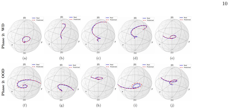
The pith
A machine-rendered reading of the paper's core claim, the machinery that carries it, and where it could break.
The reading
What carries the argument
The central object is the augmented state Y_aug(t) = [x(t), y(t), z(t), Delta(t), gamma(t)]^T, which lets a neural ODE represent both the measured Bloch trajectory and unmeasured environmental parameters. The mechanism is a measurement-conditioned latent evolution: an encoder initializes the latent trajectory from partial data, the derivative of the latent state is learned as MLP_theta([h(t), dY(t)]), and a decoder maps the latent trajectory back to physical observables and parameters. This construction allows the network to integrate measurement information over time, acting as a learned filter rather than a fixed analytical model.
What would settle it
Feed the trained model a simulated measurement trace with random shot noise added to the detector output rather than the clean trace of Eq. (7), then compare the reconstructed Bloch state to the true state; if the error rises well above the reported MSE and does not converge over time, the claim that AQNODE filters real measurement data fails.
Extended reading notes
Core claim
The paper's central claim is that a single learned augmented neural ODE can replace explicit physical equations for both state estimation and feedback control of a dissipative qubit. The model uses an augmented state Y_aug(t) = [x(t), y(t), z(t), Delta(t), gamma(t)] that includes both the observable Bloch components and the hidden time-dependent environmental parameters. Initial conditions and partial measurement outputs are encoded into a latent state, evolved by a neural ODE whose derivative function is an MLP conditioned on the measurement record, and decoded back into the physical variables. Trained on trajectories generated from a non-Markovian Lindblad master equation, the model recons
Load-bearing premise
The whole demonstration assumes the weak-measurement signal is a clean, deterministic function of the true state and that the training labels come from the same master equations that define the task, so real measurement noise or a different environment model could break it.
Editorial extensions
If this is right
- A trained AQNODE can act as an observer for dissipative qubits when the Hamiltonian or Liouvillian is unknown: from partial measurement records it outputs both the Bloch state and the hidden time-dependent decoherence parameters.
- The learned state estimate is usable for real-time closed-loop control; the paper's LQR implementation solves a differential Riccati equation using AQNODE predictions and achieves high-fidelity transfer to the target state even out of distribution.
- Initial-state perturbations decay over time as the measurement record is integrated, indicating behavior consistent with quantum filtering and suggesting practical robustness to uncertain starting conditions.
- The differentiable, adjoint-trained model can in principle be retrained or fine-tuned for new device parameters or multi-qubit systems whenever suitable trajectory data become available.
- The latent representation separates trajectories by control strategy and distributional regime, suggesting the model captures physically meaningful hidden structure rather than memorizing individual trajectories.
Reading between the lines
- The paper's validation uses a clean, deterministic measurement record; a natural stronger test is to feed the model stochastic homodyne trajectories with explicit shot noise and compare its reconstructions against a standard Bayesian quantum filter.
- Because the ground-truth parameters are generated from one specific spectral-density model, a sharper test of the 'no explicit physical equations' claim would train on that model and test on a different environment model; success would indicate the latent dynamics capture generic dissipative structure.
- The PD and LQR gains are fixed rather than globally optimized; an implicit next step is to use AQNODE's differentiability to optimize control fields end-to-end, which could close the small predicted-versus-real energy and fidelity gaps.
- AQNODE is currently a point estimator; extending it to output a posterior distribution over states and parameters would connect it more directly to established quantum filtering theory.
Editorial analysis
A structured set of objections, weighed in public.
Referee Report
Summary. The paper proposes an Augmented Quantum Neural ODE (AQNODE) framework for a single dissipative qubit. The model encodes weak-measurement traces and an initial augmented state into a latent trajectory, evolves it with a neural ODE, and decodes it into the Bloch vector components and time-dependent diffusion/dissipation parameters Δ(t) and γ(t). The authors report low MSE for state and parameter prediction in within-distribution (WD) and out-of-distribution (OOD) numerical tests, and they combine AQNODE predictions with PD and time-varying LQR controllers to steer the qubit to a target state. The abstract and conclusion claim that the method enables state reconstruction and parameter inference without explicit physical equations and that it functions as a data-driven quantum observer.
Significance. The architecture is a reasonable and potentially useful extension of latent Neural ODEs to open quantum systems, and the control comparison (PD vs LQR) is clearly presented. If the claims were validated under realistic stochastic weak measurements and with hidden initial parameters not provided to the model, AQNODE could be an attractive data-driven observer for quantum filtering and feedback control. As it stands, however, the evidence supports a narrower claim: accurate supervised trajectory fitting for a single-qubit Lindblad model when the true initial Δ(0), γ(0) are given and the measurement record is a noise-free deterministic function of the state. The current experiments do not demonstrate parameter inference from the measurement trace alone, nor do they test robustness to measurement noise or model misspecification.
major comments (4)
- [Sec. II, Eq. (7)] The measurement model is deterministic and noiseless: dY/dt = sqrt(M) ζ tr(-σ_z ρ_t) = -sqrt(M) ζ z(t). This is a continuous noise-free observation of the Bloch component z(t), not a stochastic weak-measurement record. Standard quantum filtering requires a stochastic master equation with innovations noise and measurement backaction. Feedthis deterministic trace as the network input means the claimed 'robust quantum filtering' and 'partial continuous measurement data' performance is untested for realistic noisy measurements. The authors should either reformulate Eq. (7) as a proper stochastic measurement model or explicitly restrict the claims to noiseless continuous observation.
- [Sec. III.A.1, III.A.2, IV.B] The parameter-inference claim is undermined by initialization leakage. The encoder is h(t0) = Encoderψ([Yaug(t0), dY(t)0:tk]) with Yaug(t0) = [x0,y0,z0,Δ(0),γ(0)], and each training sample includes the true initial augmented state. The Phase-2 perturbation study perturbs the full 5D vector, including Δ0 and γ0, so the model is always given the true (or perturbed-but-known) initial values of the hidden parameters. The low MSEs for Δ(t) and γ(t) in Tables I and II can therefore be explained by learning a mapping from these initial values to their future values, not by inferring them from the measurement trace. This directly contradicts the abstract's 'parameter inference without explicit physical equations.' The manuscript itself acknowledges in Sec. III.A.4 that environmental parameters 'cannot be directly measured and may require additional steps or calibration.' The model must be tested
- [Tables I, II; Sec. IV.A] Tables I and II report single MSE values, although the text states that the reported values are 'mean and standard deviation' over all test trajectories. No error bars, standard deviations, or number of test trajectories are given. Given the large OOD degradation in Phase 2 (e.g., MSE_y from 1.16×10^-3 to 5.80×10^-2), statistical quantification is essential for the generalization claim. In addition, the text in Sec. IV.A says 'the use of a physics-informed loss function ensured that the model respected the underlying physical laws,' but Eqs. (12)–(14) define the training loss as a weighted MSE only; no physics residual term is defined. Either define the physics-informed term or remove that claim.
- [Table III; Sec. IV.C] The control evaluation metrics in Table III are not clearly defined. The column 'MSE' is ambiguous: if it is the error between predicted and true controlled trajectories, then the rows 'Real PD' and 'Real LQR' should not have an MSE. 'Energy Dev' is not defined. The text also states that the predicted LQR maintains 'high fidelity (≥0.94) even under OOD conditions,' but Table III reports OOD Pred LQR fidelity as 0.932. These inconsistencies need to be resolved, and the exact formulas for MSE, final-state deviation, and fidelity should be given.
minor comments (5)
- [Sec. II, Eq. (5)] Typo in the first equation: '−(∆(t) + M/2)(t)' should likely be '−(∆(t) + M/2)x(t)'.
- [Sec. II, Eq. (7) and Sec. III.A.1] The notation is confusing: Eq. (7) defines dY/dt, but the encoder and neural ODE use dY(t) as an input. Please clarify whether the network receives the measurement trace Y(t), its derivative dY/dt, or both, and specify the sign convention tr(-σ_z ρ_t) = -z(t).
- [Sec. IV.C, target state] The target is described as the 'pure excited state' Y_target = [0,0,1], but Fig. 12 calls it the eigenstate |0>. In the standard convention |0> is the ground state. Please align the notation.
- [General] The term 'out-of-distribution' is used for parameter values drawn from wider intervals of the same parametric family (Eqs. 2-3). This is extrapolation within a family, not distribution shift to a different physical model. Consider using 'extrapolation' or 'wider-range' to avoid overstatement.
- [Appendix B, Fig. 17] The convergence shown under initial-state perturbations reflects the intrinsic stability of the Lindblad dynamics, not necessarily the filtering capability of AQNODE. This point should be stated explicitly so the perturbation experiment is interpreted correctly.
Circularity Check
No significant circularity: the AQNODE is a supervised surrogate with a standard train/test split; parameter predictions are not equivalent to inputs by construction.
full rationale
The paper's claimed derivation chain is an ML training procedure: simulate trajectories from Eq. (1) with Δ(t),γ(t) from Eqs. (2)-(3), train a latent neural ODE to map initial conditions and measurement traces to those trajectories, and evaluate MSE on unseen WD/OOD parameter draws. This is a conventional generalization claim, not a derivation of Δ(t),γ(t) from the same quantities. The apparent leakage of 'true hidden initial values' into the encoder (Sec. III.A.1: h(t0)=Encoderψ([Yaug(t0), dY(t)0:tk]) with Yaug(t0)=[x0,y0,z0,Δ(0),γ(0)]) is not circular: Eqs. (2)-(3) give Δ(0)=γ(0)=0 for every trajectory, so these inputs carry no information about the environmental parameters α,r,ω0; the actual information source is the measurement trace dY(t). The perturbation study (Sec. IV.B) perturbs Δ0,γ0 artificially, but this is a robustness test, not a claim that the true initial values are inferred. The paper itself flags the practical limitation that environmental parameters may need calibration (Sec. III.A.4), which undercuts the abstract's 'without explicit physical equations' phrasing, but this is an overstatement about experimental readiness, not a circular step. No load-bearing self-citation or imported uniqueness theorem is used; ref. [42] is a standard citation for the Lindblad form. The in-sample evaluation on the same generative family limits external validity, but it is not circularity.
Assumptions & free parameters
free parameters (4)
- Loss weights κ and β =
unspecified
- PD controller gains =
kxp=5, kyp=10, kxd=8, kyd=10
- LQR weights Q and R =
Q=diag(1000,1000,1000), R=diag(0.1,50)
- Network architecture sizes =
encoder/ODE/decoder MLP sizes not fully specified; ~130k parameters in phase 1, 51,976 in phase 3
assumptions (4)
- domain assumption The Lindblad master equation (Eq. 1) is the exact generator of the qubit dynamics, with time-dependent Δ(t) and γ(t) given by Eqs. (2)-(3).
- ad hoc to paper The weak measurement output dY(t)/dt = sqrt(M) ζ tr(-σz ρ_t) is a noise-free deterministic function of the state (Eq. 7).
- domain assumption The latent state h(t) ∈ R^d initialized by an encoder and evolved by an MLP parameterizes the full augmented state [x,y,z,Δ,γ] through a decoder.
- domain assumption The analytical forms of Δ(t) and γ(t) (Eqs. B5-B7) are the only source of non-Markovianity; training and test trajectories are drawn from this family.
Cite this review
Pith. "Pith review of Quantum Filtering and Stabilization of Dissipative Quantum Systems via Augmented Neural Ordinary Differential Equations." pith.science (2026). https://pith.science/paper/37I66E5U
@misc{pith2026250907196,
  author       = {Pith},
  title        = {Pith review of: Quantum Filtering and Stabilization of Dissipative Quantum Systems via Augmented Neural Ordinary Differential Equations},
  year         = {2026},
  howpublished = {\url{https://pith.science/paper/37I66E5U}},
  note         = {Machine review of arXiv:2509.07196}
}
read the original abstract
Modeling open quantum dynamics without full knowledge of the system Hamiltonian or noise model is a key challenge in quantum control and quantum state estimation. We introduce an Augmented Quantum Neural Ordinary Differential Equation (AQNODE) framework that learns quantum trajectories and dissipation parameters directly from partial continuous measurement data. By embedding the system into a latent space evolved via neural ODEs, AQNODE captures both observable and hidden non-Markovian dynamics with temporal smoothness and physical consistency. Our approach integrates weak measurement data to reconstruct qubit states and time-dependent decoherence rates, enabling accurate state prediction and parameter inference without explicit physical equations. Furthermore, we incorporate AQNODE-based feedback control techniques, including proportional-derivative and time-varying linear-quadratic regulator (LQR) strategies, to steer the quantum system toward target states in real time. Extensive numerical simulations demonstrate AQNODE's ability to generalize across system configurations, achieve low prediction errors, and perform robust quantum filtering and control. These results establish AQNODE as a scalable, differentiable, and experimentally compatible framework for real-time modeling and control of dissipative quantum systems.
Figures


Figures from the paper (14 more)




Reference graph
Works this paper leans on
-
[1]
Latent Dynamics:Once initialized, the latent state evolves via a neural ODE
Dynamics of Augmented System Since direct access toY aug(t) is generally unavail- able, we initialize a latent trajectoryh(t)∈R d 5 from partial data using an encoder network:h(t 0) = Encoderψ ([Yaug(t0), dY(t)0:tk ]), where Encoder ψ is a learnable neural network parameterized byψ. Latent Dynamics:Once initialized, the latent state evolves via a neural O...
-
[2]
1) over a time intervalt∈[0, T) and with the continuous weak measurementY(t)
Data Generation The training dataset is generated by simulating the evolution of a single qubit system under a non-Markovian open quantum dynamics governed by a time-dependent Lindblad equation (Eq. 1) over a time intervalt∈[0, T) and with the continuous weak measurementY(t). For each trajectory, the dissipation strengthα, memory pa- rameterr, system-envi...
-
[3]
Learning Process An MLP is employed to represent the dynamical rule of the latent state in the neural ODE framework. The latent space dimension determines the representation’s complexity, which allows the model to describe compli- cated system dynamics. The training procedure of AQN- ODE is: Initialization: The initial encoder latent state (h 0) and the m...
-
[4]
Training The training procedure for learning quantum dynam- ics using Neural ODEs involves simulating the dissipative Bloch equations to generate ground truth trajectories 6 and training a neural network to reconstruct these trajec- tories from weak measurement data. A decoder is used to translate the enhanced latent representation of the sys- tem’s state...
-
[5]
Validation After training, the model is evaluated on two differ- ent test datasets: within-distribution (WD) testing and out-of-distribution (OOD) testing and with different per- turbations in the initial qubit state. The WD test set consists of qubit trajectories generated using parameter ranges similar to the training set, while the OOD test set include...
-
[6]
LQR Control To achieve optimal control of the quantum state, LQR control dynamically adjusts feedback gains based on a cost function [49, 52]. The evolution of the Bloch vec- tor is governed by the ˆY(t) = [ˆx(t),ˆy(t),ˆz(t)]T , and the control fieldsu x(t), uy(t) are applied via the Hamiltonian operatorsA x andA y. Thus, the control matrixB(t) is constru...
-
[7]
Phase 3: PD control The PD control strategy computes the control fields based on the error ( ˆY(t)− Ytarget) and its derivative ˙ˆY(t) [53, 54]. Then the control fields are calculated as ux =−k x p ·e x(t)−k x d · ˙ˆx(t) (20) uy =−k y p ·e y(t)−k y d · ˙ˆy(t) (21) The errorse x(t) = ˆx(t)−x target(t) ande y(t) = ˆy(t)− ytarget(t) between the current estim...
-
[8]
Preliminaries of state transfer Coherence and purity are essential markers of the dy- namics of quantum systems. Pure (p(t) = 1) and mixed (p(t)<1) quantum states are distinguished by purity, i.e.,p(t) = 1+x2(t)+y2(t)+z2(t) 2 , which reflects the degree of decoherence or dissipation in the system. Its temporal evolution shows how energy splitting (∆(t)) a...
Show all 62 references
-
[9]
Gebhart, R
V. Gebhart, R. Santagati, A. A. Gentile, E. M. Gauger, D. Craig, N. Ares, L. Banchi, F. Marquardt, L. Pezze, and C. Bonato, Learning quantum systems, Nature Re- views Physics5, 141 (2023)
2023
-
[10]
Havl ´ ıˇ cek, A
V. Havl ´ ıˇ cek, A. D. C´ orcoles, K. Temme, A. W. Harrow, A. Kandala, J. M. Chow, and J. M. Gambetta, Super- vised learning with quantum-enhanced feature spaces, Nature567, 209 (2019)
2019
-
[11]
I. R. Petersen and D. Dong, Special section on estimation and control of quantum systems (2022)
2022
-
[12]
Mart ´ ınez-Vargas, C
E. Mart ´ ınez-Vargas, C. Pineda, F. Leyvraz, and P. Barberis-Blostein, Quantum estimation of unknown parameters, Physical Review A95, 012136 (2017)
2017
-
[13]
Cortez, A
L. Cortez, A. Chantasri, L. P. Garc ´ ıa-Pintos, J. Dressel, and A. N. Jordan, Rapid estimation of drifting parame- ters in continuously measured quantum systems, Physical Review A95, 012314 (2017)
2017
-
[14]
H. Liao, D. S. Wang, I. Sitdikov, C. Salcedo, A. Seif, and Z. K. Minev, Machine learning for practical quantum error mitigation, Nature Machine Intelligence6, 1478 (2024)
2024
-
[15]
J. B. Rigo and A. K. Mitchell, Machine learning effective models for quantum systems, Physical Review B101, 241105 (2020)
2020
-
[16]
LeCun, Y
Y. LeCun, Y. Bengio, and G. Hinton, Deep learning, Na- ture521, 436 (2015)
2015
-
[17]
Huang, R
H.-Y. Huang, R. Kueng, and J. Preskill, Predicting many properties of a quantum system from very few measure- ments, Nature Physics16, 1050 (2020)
2020
-
[18]
H. Ma, B. Qi, I. R. Petersen, R.-B. Wu, H. Rabitz, and D. Dong, Machine learning for estimation and control of quantum systems, National Science Review , nwaf269 (2025)
2025
-
[19]
M. Y. Niu, S. Boixo, V. N. Smelyanskiy, and H. Neven, Universal quantum control through deep reinforcement learning, npj Quantum Information5, 33 (2019)
2019
-
[20]
Preskill, Quantum computing in the nisq era and be- yond, Quantum2, 79 (2018)
J. Preskill, Quantum computing in the nisq era and be- yond, Quantum2, 79 (2018)
2018
-
[21]
Callison and N
A. Callison and N. Chancellor, Hybrid quantum-classical algorithms in the noisy intermediate-scale quantum era and beyond, Physical Review A106, 010101 (2022)
2022
-
[22]
Bharti, A
K. Bharti, A. Cervera-Lierta, T. H. Kyaw, T. Haug, S. Alperin-Lea, A. Anand, M. Degroote, H. Heimonen, J. S. Kottmann, T. Menke,et al., Noisy intermediate- scale quantum algorithms, Reviews of Modern Physics 94, 015004 (2022)
2022
-
[23]
H. M. Wiseman and G. J. Milburn,Quantum measure- ment and control(Cambridge university press, 2009)
2009
-
[24]
M. A. Nielsen and I. L. Chuang,Quantum computation and quantum information(Cambridge university press, 2010)
2010
-
[25]
Domingo, G
L. Domingo, G. Carlo, and F. Borondo, Optimal quan- tum reservoir computing for the noisy intermediate-scale quantum era, Physical Review E106, L043301 (2022)
2022
-
[26]
M. J. Ranˇ ci´ c, Noisy intermediate-scale quantum comput- ing algorithm for solving an n-vertex maxcut problem with log (n) qubits, Physical Review Research5, L012021 (2023)
2023
-
[27]
H. M. Wiseman and G. J. Milburn, Quantum theory of optical feedback via homodyne detection, Physical Re- view Letters70, 548 (1993)
1993
-
[28]
T. H. Kyaw, T. Menke, S. Sim, A. Anand, N. P. Sawaya, W. D. Oliver, G. G. Guerreschi, and A. Aspuru-Guzik, Quantum computer-aided design: digital quantum sim- ulation of quantum processors, Physical Review Applied 16, 044042 (2021)
2021
-
[29]
Iyer and D
P. Iyer and D. Poulin, A small quantum computer is needed to optimize fault-tolerant protocols, Quantum Science and Technology3, 030504 (2018)
2018
-
[30]
V. M. Bastidas, T. H. Kyaw, J. Tangpanitanon, G. Romero, L.-C. Kwek, and D. G. Angelakis, Flo- quet stroboscopic divisibility in non-markovian dynam- ics, New Journal of Physics20, 093004 (2018)
2018
-
[31]
T. H. Kyaw, D. A. Herrera-Marti, E. Solano, G. Romero, and L.-C. Kwek, Creation of quantum error correcting codes in the ultrastrong coupling regime, Physical Re- view B91, 064503 (2015)
2015
-
[32]
K. R. Brown, J. Kim, and C. Monroe, Co-designing a scalable quantum computer with trapped atomic ions, npj Quantum Information2, 1 (2016)
2016
-
[33]
De Vega and D
I. De Vega and D. Alonso, Dynamics of non-markovian open quantum systems, Reviews of Modern Physics89, 015001 (2017)
2017
-
[34]
Flannigan, F
S. Flannigan, F. Damanet, and A. J. Daley, Many-body quantum state diffusion for non-markovian dynamics in strongly interacting systems, Physical Review Letters 128, 063601 (2022)
2022
-
[35]
V. R. Overbeck and H. Weimer, Time evolution of open quantum many-body systems, Physical Review A93, 012106 (2016)
2016
-
[36]
Biamonte, P
J. Biamonte, P. Wittek, N. Pancotti, P. Rebentrost, N. Wiebe, and S. Lloyd, Quantum machine learning, Na- ture549, 195 (2017)
2017
-
[37]
R. Iten, T. Metger, H. Wilming, L. Del Rio, and R. Ren- ner, Discovering physical concepts with neural networks, Physical Review Letters124, 010508 (2020)
2020
-
[38]
Flam-Shepherd, T
D. Flam-Shepherd, T. C. Wu, X. Gu, A. Cervera-Lierta, M. Krenn, and A. Aspuru-Guzik, Learning interpretable representations of entanglement in quantum optics ex- periments using deep generative models, Nature Machine Intelligence4, 544 (2022)
2022
-
[39]
R. T. Chen, Y. Rubanova, J. Bettencourt, and D. K. Du- venaud, Neural ordinary differential equations, Advances in Neural Information Processing Systems31(2018). 20
2018
-
[40]
Dupont, A
E. Dupont, A. Doucet, and Y. W. Teh, Augmented neu- ral odes, Advances in Neural Information Processing Sys- tems32(2019)
2019
-
[41]
M. Choi, D. Flam-Shepherd, T. H. Kyaw, and A. Aspuru- Guzik, Learning quantum dynamics with latent neural ordinary differential equations, Physical Review A105, 042403 (2022)
2022
-
[42]
Chen and Y
L. Chen and Y. Wu, Learning quantum dissipation by the neural ordinary differential equation, Physical Review A 106, 022201 (2022)
2022
-
[43]
J. Li, X. Yang, X. Peng, and C.-P. Sun, Hybrid quantum- classical approach to quantum optimal control, Physical Review Letters118, 150503 (2017)
2017
-
[44]
S. C. Hou, M. A. Khan, X. X. Yi, D. Dong, and I. R. Petersen, Optimal lyapunov-based quantum control for quantum systems, Physical Review A86, 022321 (2012)
2012
-
[45]
Campagne-Ibarcq, E
P. Campagne-Ibarcq, E. Flurin, N. Roch, D. Darson, P. Morfin, M. Mirrahimi, M. H. Devoret, F. Mallet, and B. Huard, Persistent control of a superconducting qubit by stroboscopic measurement feedback, Physical Review X3, 021008 (2013)
2013
-
[46]
Lloyd and J.-J
S. Lloyd and J.-J. E. Slotine, Quantum feedback with weak measurements, Physical Review A62, 012307 (2000)
2000
-
[47]
Zhang, Y
J. Zhang, Y. xi Liu, R.-B. Wu, K. Jacobs, and F. Nori, Quantum feedback: Theory, experiments, and applica- tions, Physics Reports679, 1 (2017), quantum feedback: theory, experiments, and applications
2017
-
[48]
Yang and Z
L. Yang and Z. Shao, Neural controlled differen- tial equations with quantum hidden evolutions (2024), arXiv:2404.19673 [cs.LG]
2024 arXiv
-
[49]
W. Cui, Z. R. Xi, and Y. Pan, Optimal decoherence control in non-markovian open dissipative quantum sys- tems, Physical Review A—Atomic, Molecular, and Opti- cal Physics77, 032117 (2008)
2008
-
[50]
Qamar, S
S. Qamar, S. Cong, K. Li, Z. Dong, and F. Shuang, Non- linear optimal feedback control of the two-level open non- markovian stochastic quantum system, Open Systems & Information Dynamics28, 2150013 (2021)
2021
-
[51]
Breuer, E.-M
H.-P. Breuer, E.-M. Laine, J. Piilo, and B. Vacchini, Col- loquium: Non-markovian dynamics in open quantum sys- tems, Reviews of Modern Physics88, 021002 (2016)
2016
-
[52]
Maniscalco, S
S. Maniscalco, S. Olivares, and M. G. Paris, Entan- glement oscillations in non-markovian quantum chan- nels, Physical Review A—Atomic, Molecular, and Op- tical Physics75, 062119 (2007)
2007
-
[53]
Gardiner and P
C. Gardiner and P. Zoller,Quantum noise: a handbook of Markovian and non-Markovian quantum stochastic meth- ods with applications to quantum optics(Springer Science & Business Media, 2004)
2004
-
[54]
G. E. Fux, E. P. Butler, P. R. Eastham, B. W. Lovett, and J. Keeling, Efficient exploration of hamiltonian pa- rameter space for optimal control of non-markovian open quantum systems, Physical Review Letters126, 200401 (2021)
2021
-
[55]
Hwang and H.-S
B. Hwang and H.-S. Goan, Optimal control for non- markovian open quantum systems, Physical Review A—Atomic, Molecular, and Optical Physics85, 032321 (2012)
2012
-
[56]
Wu and W
S. Wu and W. Ma, Trajectory tracking for non-markovian quantum systems, Physical Review A105, 012204 (2022)
2022
-
[57]
S. C. Edwards and V. P. Belavkin, Optimal quantum filtering and quantum feedback control, arXiv preprint quant-ph/0506018 (2005)
2005 arXiv
-
[58]
Langen, G
T. Langen, G. Valtolina, D. Wang, and J. Ye, Quantum state manipulation and cooling of ultracold molecules, Nature Physics20, 702 (2024)
2024
-
[59]
Ryan-Anderson, J
C. Ryan-Anderson, J. G. Bohnet, K. Lee, D. Gresh, A. Hankin, J. Gaebler, D. Francois, A. Chernoguzov, D. Lucchetti, N. C. Brown,et al., Realization of real-time fault-tolerant quantum error correction, Physical Review X11, 041058 (2021)
2021
-
[60]
A. C. Doherty and K. Jacobs, Feedback control of quan- tum systems using continuous state estimation, Physical Review A60, 2700 (1999)
1999
-
[61]
H. Chen, H. Li, F. Motzoi, L. Martin, K. B. Whaley, and M. Sarovar, Quantum proportional-integral (pi) control, New Journal of Physics22, 113014 (2020)
2020
-
[62]
J. E. Gough, A quantum kalman filter-based pid con- troller, Open Systems & Information Dynamics27, 2050014 (2020)
2020
Reviewed August 4, 2026 · model on record in the stance chip above.
Discussion (0). Sign in to comment.