REVIEW 3 major objections 5 minor 5 references
Microlocal analysis of the non-relativistic limit of the Klein--Gordon equation: Estimates
T0 review · 3 major / 5 minor · reviewed 2026-08-04 · deepseek-v4-flash
Pith's one-line read This paper proves that the Klein–Gordon operator on asymptotically Minkowski spacetimes is invertible between carefully chosen Sobolev spaces with a bound that stays finite as the speed of light c tends to infinity, making the non-relativis
desk verdict A serious technical paper that builds three new calculi to get uniform-in-c Fredholm control of Klein-Gordon, but the closing remainder estimate leans on a deferred adaptation of the GRGH22 Schrödinger result and should go to referees only with that appendix fully available. read the letter →
The pith
A machine-rendered reading of the paper's core claim, the machinery that carries it, and where it could break.
The reading
What carries the argument
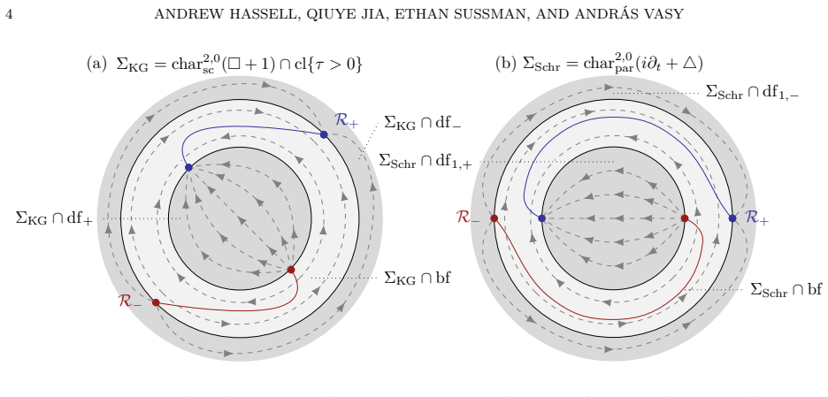
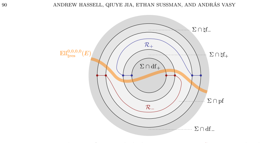
Three new pseudodifferential calculi, Ψ♮, Ψ♮res, and Ψ♮2res, built by second-microlocalizing at the two natural frequencies (τ♮,ξ♮)=(±1,0). The twice-resolved phase space has boundary faces df (fiber infinity), bf (spacetime infinity), ♮f (natural face), and pf± (parabolic faces); the normal operator of P± at pf± is the Schrödinger operator, which is the mechanism that converts the Klein–Gordon problem into two Schrödinger problems in the limit. The central structural fact is that the ♮2res-Hamiltonian flow is globally source-to-sink in the relevant component Σ of the characteristic set, which lets propagation and radial-point estimates hold uniformly in h=c^{-1} and close the Fredholm argum
What would settle it
Compute, for the exactly soluble case d=1 with a constant coefficient Klein–Gordon operator and a fixed Gaussian source f, the sequence of solutions u_c. The theorem predicts that the microlocalized projections onto the two parabolic faces, after removal of the oscillations e^{±ic^2t}, are governed by the free Schrödinger equation, with the remainder in the ♮2res norm of order (0,0,1;0,0) decaying as c→∞. A numerical or symbolic calculation showing that the remainder stays O(1), or that the ratio ||u_c||/||f|| grows without bound, would contradict Theorem 1.1.
Extended reading notes
Core claim
On the twice-resolved natural phase space, whose boundary has faces at fiber infinity, spacetime infinity, the natural face, and two parabolic faces pf±, the conjugated Klein–Gordon family P± has principal symbol whose rescaled Hamiltonian flow is source-to-sink within the good sheet Σ of the characteristic set, with radial sets R± lying over past and future spacetime infinity. Theorem 1.1 states that, for a variable order s that is monotone along this flow and satisfies s>−1/2 on one radial set and s<−1/2 on the other, plus two technical conditions, P is an invertible map X^{m,s,ℓ}→Y^{m−1,s+1,ℓ−1} for all c>c0 with a uniform bound on the inverse. The estimate closes by combining propagation
Load-bearing premise
The proof depends on a uniform half-Fredholm estimate for the Schrödinger operator, imported from a previous analysis of the parabolic calculus, holding for variable orders pulled back from the twice-resolved phase space; if that estimate does not survive the pull-back, the remainder bound in §5.3 fails and Theorem 1.1 collapses.
Editorial extensions
If this is right
- For any smooth, compactly supported forcing f that is uniformly bounded in c, the solution P^{-1}f lies in H^{1,s,1;0,0}_{♮2res}, which has order 1 (i.e. O(c^{-1})) at the natural face and order 0 at the parabolic faces, confirming that the Schrödinger operator governs the leading asymptotic behaviour.
- The uniform bound allows one to pass to the limit c→∞ in the estimates, yielding that the c=∞ behaviour decouples into two copies of the Schrödinger flow, one per sign of the energy.
- The construction yields four distinct global inverses—forward, backward, Feynman, and anti-Feynman solutions—distinguished by whether the variable decay order s is above or below the threshold -1/2 at the radial sets.
- The two technical conditions on s (constancy near radial sets and smoothness of |H_p s|^{1/2}) are stated as removable via the sharp Gårding inequality, so the essential threshold is just the monotonicity and the ±1/2 condition.
- Intermediate frequencies at corners pf±∩♮f and very large frequencies at ♮f∩df are controlled, showing that only laboratory and natural scales are required for the solvability theory.
Reading between the lines
- A testable extension: the same twice-resolved scheme should apply to the Dirac and Proca equations, where the non-relativistic limit also produces two Schrödinger-like branches; the role of the two parabolic faces would be played by the two spin or charge branches.
- A numerical check: solve the Klein–Gordon equation in d=1 with a time-independent potential for a sequence of increasing c and fixed smooth source; the theorem predicts the ratio of the solution in the ♮2res norm to the source norm stays bounded, and that the projected solution at frequencies near ±c^2 follows the Schrödinger evolution with error O(c^{-1}) in the stated norm.
- The authors' Remark 1.3 suggests the variable order is a technical tool; if the sharp Gårding adaptation works, the allowed decay orders form an open set around -1/2, so any physically reasonable decaying source is covered.
- If the uniform estimate holds, it implies a resolvent-type convergence: for time-harmonic sources with frequency near ±c^2+O(1), the solution's leading term should equal the Schrödinger resolvent; failure of such resolvent convergence would provide a sharp falsifier.
Editorial analysis
A structured set of objections, weighed in public.
Referee Report
Summary. The paper develops three new pseudodifferential calculi—Ψ♮, Ψ♮res, and Ψ♮2res—designed to analyze the Klein–Gordon operator as the speed of light c tends to infinity. The main result, Theorem 1.1 (eqs. (1.13)–(1.14)), asserts uniform invertibility of a class of Klein–Gordon-type operators between anisotropic Sobolev spaces associated with the twice-resolved natural phase space, provided a variable order s satisfies monotonicity and threshold conditions relative to the two radial sets in each component of the characteristic set. The proof strategy is to study the conjugated operators P± of §3, compute the characteristic set and radial-point dynamics in §4, and then close a chain of elliptic, propagation, radial-point, and remainder estimates in §5. The normal operator at the parabolic face is the nonrelativistic Schrödinger operator, so the final remainder estimate imports the half-Fredholm theory of Gell-Redman–Gomes–Hassell. The paper is the technical companion to an applications paper and is explicitly written to be usable as a black box.
Significance. If the main theorem is fully established, this would be a substantial and useful contribution: it provides a uniform-in-c microlocal framework that interpolates between the scattering calculus for the Klein–Gordon equation and the parabolic calculus for the Schrödinger equation, and it makes precise the heuristic that the nonrelativistic limit is governed by two copies of the Schrödinger flow (eq. (1.10)). The paper contains real technical achievements, including explicit characteristic-set and radial-set computations (§4), normal-operator computations (§3.2), and a multi-graded composition law for the new calculi (§2.5–2.6). The result has no fitted parameters; the threshold −1/2 is dictated by the radial-point dynamics (Prop. 4.17), and the monotonicity hypotheses are explicit. The principal weakness is that the estimate chain closes only through Lemma 5.9, whose proof depends on an adaptation of [GRGH22] that is deferred to Appendix B; in the text available for review, that appendix is truncated, and §5.4 is also not present. These are missing-support concerns rather than demonstrated errors.
major comments (3)
- [§5.3, Lemma 5.9, eq. (5.69)] This lemma is load-bearing: it provides the remainder estimate that closes the chain (5.1). The statement requires a uniform-in-h, variable-order, half-Fredholm estimate for the Schrödinger normal operator N(P±), with the pulled-back order s|pf+ε, with constants independent of ε, and with the incoming/outgoing condition WF^{ℓ',s0}_{par}(Πu)∩R^{Schr}_{−ς}=∅ preserved under the microlocal cutoff O2Π. These requirements go beyond the literal statement of [GRGH22, Thm. 1.1], and the proof refers to 'the adaptation in Section B.' However, Appendix B is not present in the text made available for review. Without the actual adaptation, eq. (5.69) is unsupported, and the central estimate of Theorem 1.1 is not verified.
- [§5.4 and eq. (5.1)] The advertised final absorption step is missing. The paper's own summary of the proof, eq. (5.1), ends with an h^ε term that is absorbed into the left-hand side after the estimates for P± are combined on the two components of the characteristic set. That combination and absorption are the steps that turn the microlocal estimates for P± into the claimed global ♮2res estimate (1.14) for P. In the text under review, §5.4 is announced but not included. Hence Theorem 1.1 is not proven within the provided manuscript.
- [§5.3, proof of Lemma 5.9, eqs. (5.70)–(5.77)] Even apart from the missing appendix, the proof asserts that the variable order ̲s=s|pf+ε inherits the monotonicity required by [GRGH22] from the monotonicity of s under the ♮res Hamiltonian flow. This is plausible because pf is canonically identified with parT*M and R^{Schr}_ς corresponds to R_ς∩pf, but the implication is not proved. Since the whole argument depends on applying the Schrödinger radial-point and propagation estimates to a variable order that is only known to be constant near the radial sets and pulled back from pf, this step needs a precise statement. If [GRGH22] requires global constancy of the order near the radial sets in a neighborhood that is incompatible with the ε-regularization, the remainder estimate (5.69) would fail.
minor comments (5)
- [§1, after Theorem 1.1] The text refers to 'Proposition 1.1' in the paragraph following Theorem 1.1 and again in §1.4; the statement is a theorem, not a proposition. Please correct the cross-reference.
- [§3, eq. (3.10)] The first displayed line in (3.10) contains '1/c^5 ∂^2_t', which appears to be a typo for a term of order c^{-5} or a mismatched exponent. Please check the intended order at ♮f and pf.
- [§2.6] The numbering 'Corollary 2.19.1' is nonstandard and likely a LaTeX artifact; renumber as a numbered corollary or inline consequence.
- [§5.2, Proposition 5.10 proof] In the proof, the text says 'we may assume that WF′♮(Π) is as close to the zero section as we wish' and then takes WF′♮(Π)⊆Ell(O1). But Π is fixed in the hypothesis. The argument should explain how the given Π can be replaced by a microlocalized version, or why the estimate is independent of the choice of Π.
- [§2.2–2.3] Notation is inconsistent between ♮resT*M and ♮,resT*M in Figure 4 and a few nearby passages. Standardize the symbol for the resolved natural phase space.
Circularity Check
No significant circularity: the derivation is self-contained apart from an external Schrödinger solvability input whose adaptation is deferred but not circular.
full rationale
The paper's central claim, Theorem 1.1, is a uniform-in-c invertibility estimate for the Klein–Gordon family P. The proof chain is: construct the ♮/♮res/♮2res calculi from standard compactifications and quantization (§2), compute the characteristic set and radial set dynamics of the conjugated operators P± (§4), prove elliptic, propagation and radial point estimates in the new calculus (§5.1–5.2), and then close the remainder estimate using the Schrödinger normal operator solvability imported from [GRGH22] (§5.3, Lemma 5.9). No parameter is fitted to the target estimate and no quantity called a prediction is defined in terms of the result: the threshold −1/2 is dictated by the sign computation in Proposition 4.17, and the monotonicity/threshold hypotheses on s are explicit conditions on the input order, not hidden tuning. The c=∞ Schrödinger description, eq. (1.10), is a consequence of the way the ♮2res-Sobolev norms are defined (eq. (2.203)), i.e. it is a definition/construction rather than a circularly derived prediction of the theorem. The only potentially load-bearing external input is Lemma 5.9, which adapts the main results of [GRGH22] to the variable-order, h-uniform setting needed here. This is a genuine external theorem about the Schrödinger equation, not about the Klein–Gordon operator; although one coauthor (Hassell) is shared, the cited result is parameter-free, has stated assumptions that do not include the target KG estimate, and is not a restatement of Theorem 1.1. Under the rule that such citations count as real evidence, this does not raise the circularity score. The paper itself flags the reliance on [GRGH22] ('Here is where that input is used', §5) and defers the adaptation to Appendix B, which is truncated in the reviewed text; that is a missing-support or completeness concern, not a circularity concern. No specific equation was found that reduces to its own input by construction.
Assumptions & free parameters
free parameters (1)
- variable order s on ♮2resT*M
assumptions (5)
- domain assumption External Schrödinger solvability: the half-Fredholm estimate of [GRGH22], adapted in Appendix B, holds uniformly with the pulled-back variable order s|pf (Lemma 5.9)
- domain assumption Geometric setup: metric g(c) of form (3.2) with classical-symbol perturbations, non-trapping for each c, globally hyperbolic with t a time function and {t=0} Cauchy (§3.1)
- domain assumption L2-symmetry to leading subleading order: (3.13) and (3.14) on imaginary parts of β, Bj, W
- standard math Composition and principal-symbol short exact sequence for the new calculi (Props 2.8, 2.16, 2.29) hold with the asserted orders
- standard math Radial point threshold is exactly -1/2, with source/sink signs per Prop 4.17
invented entities (3)
-
Natural calculus Ψ♮ and phase space ♮T*M
independent evidence
-
Resolved natural calculus Ψ♮res and phase space ♮resT*M
independent evidence
-
Twice-resolved calculus Ψ♮2res and phase space ♮2resT*M with faces df, bf, ♮f, pf±
independent evidence
Cite this review
Pith. "Pith review of Microlocal analysis of the non-relativistic limit of the Klein--Gordon equation: Estimates." pith.science (2026). https://pith.science/paper/EMECQHKG
@misc{pith2026250909518,
  author       = {Pith},
  title        = {Pith review of: Microlocal analysis of the non-relativistic limit of the Klein--Gordon equation: Estimates},
  year         = {2026},
  howpublished = {\url{https://pith.science/paper/EMECQHKG}},
  note         = {Machine review of arXiv:2509.09518}
}
abstract
This is the more technical half of a two-part work in which we introduce a robust microlocal framework for analyzing the non-relativistic limit of relativistic wave equations with time-dependent coefficients, focusing on the Klein--Gordon equation. Two asymptotic regimes in phase space are relevant to the non-relativistic limit: one corresponding to what physicists call ``natural'' units, in which the PDE is approximable by the free Klein--Gordon equation, and a low-frequency regime in which the equation is approximable by the usual Schrodinger equation. Combining the analyses in the two regimes gives global estimates which are uniform as the speed of light goes to infinity. The companion paper gives applications. Our main technical tools are three new pseudodifferential calculi, $\Psi_{\natural}$ (a variant of the semiclassical scattering calculus), $\Psi_{\natural\mathrm{res}}$, and $\Psi_{\natural2\mathrm{res}}$, the latter two of which are created by ``second microlocalizing'' the first at certain locations. This paper and the companion paper can be read in either order, since the latter treats the former as a black box.
Figures


Figures from the paper (11 more)



Reference graph
Works this paper leans on
-
[4]
arXiv:2204.08355 [math.AP](cit. on p. 7). [Sus23] .Massive wave propagation near null infinity. To appear in Ann. PDE
-
[5]
arXiv:2305.01119 [math.AP](cit. on p. 7). [Vas13] A. Vasy. “Microlocal analysis of asymptotically hyperbolic and Kerr-de Sitter spaces (with an appendix by Semyon Dyatlov)”.Invent. Math.194.2 (2013), 381–513.doi: 10.1007/s00222-012-0446-8 .url: https://doi.org/10.1007/s00222-012-0446-8(cit. on p. 7). [Vas18] A. Vasy. “A minicourse on microlocal analysis f...
arXiv 2013
-
[2022]
Scattering regularity for small data solutions of the nonlinear Schrödinger equation
arXiv:2201.03140 [math.AP] (cit. on pp. 2, 7, 10, 11, 16, 35, 54, 57, 58, 69, 70, 79–81, 83, 93). [GRGH23] . “Scattering regularity for small data solutions of the nonlinear Schrödinger equation” (2023). arXiv:2305.12429 [math.AP](cit. on pp. 2, 7, 81–84). [H¨07] L. Hörmander.The analysis of linear partial differential operators. III. Classics in Mathemat...
arXiv 2023
-
[2023]
Dirac operators and local invariants on perturbations of Minkowski space
arXiv:2408.12057 [math.AP](cit. on p. 79). 98 REFERENCES [DVW24] V. Dang, A. Vasy, and M. Wrochna. “Dirac operators and local invariants on perturbations of Minkowski space” (2024). arXiv:2412.12714 [math.AP](cit. on p. 7). [DZ16] S. Dyatlov and M. Zworski. “Dynamical zeta functions for Anosov flows via microlocal analysis”.Ann. Sci. Éc. Norm. Supér. (4)4...
arXiv 2024
-
[2024]
Asymptotics of radiation fields in asymptotically Minkowski space
arXiv:2409.01134 [math.AP](cit. on p. 7). [BVW15] D. Baskin, A. Vasy, and J. Wunsch. “Asymptotics of radiation fields in asymptotically Minkowski space”. Amer. J. Math.137.5 (2015), 1293–1364.doi:10.1353/ajm.2015.0033(cit. on p. 7). [CH23] T. Candy and S. Herr.The massless and the non-relativistic limit for the cubic Dirac equation
arXiv 2015
Reviewed August 4, 2026 · model on record in the stance chip above.
Discussion (0). Continue with ORCID to comment.