REVIEW 3 major objections 4 minor 28 references
From the Gradient-Step Denoiser to the Proximal Denoiser and their associated convergent Plug-and-Play algorithms
T0 review · 3 major / 4 minor · reviewed 2026-08-15 · deepseek-v4-flash
Pith's one-line read A denoiser trained as a gradient step or proximal operator can be plugged into PGD or Douglas-Rachford splitting to produce iterates that provably converge to a stationary point of an explicit objective.
desk verdict A useful, honest parameter study of the authors' own convergent PnP algorithms; the theory is restated accurately, but the trained Prox denoiser's contraction property is never measured, so the 'convergent' label stays conditional. read the letter →
The pith
A machine-rendered reading of the paper's core claim, the machinery that carries it, and where it could break.
The reading
What carries the argument
The load-bearing object is the Gradient-Step denoiser $D_\sigma = \mathrm{Id}-\nabla g_\sigma$, built from $g_\sigma(x)=\frac{1}{2}\|x-N_\sigma(x)\|^2$; computing it costs one forward and one backward pass through $N_\sigma$, and because it is a gradient field the implicit prior becomes explicit. The companion identity is Proposition 3.1: if $\nabla g_\sigma$ is $L$-Lipschitz with $L<1$, then $D_\sigma = \mathrm{Prox}_{\varphi_\sigma}$ for the explicit weakly convex potential given above, so a contracted gradient-step denoiser is a true proximity operator. The contraction itself is trained by softly penalizing the spectral norm of $J(\mathrm{Id}-D_\sigma)$ with $\max(\||J(\mathrm{Id}-D_\sigma)\||,1-\varepsilon)$ via power iteration. These identities are what carry the argument: they convert the Plug-and-Play fixed-point iteration into a proximal splitting of a known functional, bringing standard nonconvex optimization convergence machinery to bear.
What would settle it
Take the released Prox-DRUNet checkpoint, compute the power-iteration estimate of $\||J(\mathrm{Id}-D_\sigma)\||$ on a batch of natural images, and compare it with 1 and with 1/2. If the estimate exceeds those thresholds at points the algorithms visit, the hypotheses of Theorems 3.1-3.3 fail there, and one can then check whether the residual still follows the announced $O(1/\sqrt{K})$ rate and whether $F$ remains nonincreasing.
Extended reading notes
Core claim
The central claim is that the gradient-step identity $D_\sigma = \mathrm{Id} - \nabla g_\sigma$, with $g_\sigma(x)=\frac{1}{2}\|x-N_\sigma(x)\|^2$, turns a trained denoiser into a gradient of an explicit regularizer, so the Plug-and-Play fixed point solves the explicit problem $\min \frac{1}{\lambda}f + g_\sigma$. When $\nabla g_\sigma$ is $L$-Lipschitz with $L<1$, the same operator is exactly $\mathrm{Prox}_{\varphi_\sigma}$ for the explicit weakly convex potential $\varphi_\sigma(x)=g_\sigma(D_\sigma^{-1}(x))-\frac{1}{2}\|D_\sigma^{-1}(x)-x\|^2+K$, and this unlocks Douglas-Rachford variants whose convergence needs no condition on $\lambda$. With these identities in place, the convergence theorems in Sections 2.3 and 3.3 guarantee monotone decrease of a computable objective, residual convergence at rate $O(1/\sqrt{K})$, and stationarity of cluster points; the paper's experiments confirm the rate and map out the role of $\sigma$, $\lambda$, and $tau_0$.
Load-bearing premise
The convergence theorems assume the trained network's $\nabla g_\sigma$ is $L$-Lipschitz with $L<1$ (or $L<1/2$ for Prox-PnP-DRS), but the training loss only softly penalizes the spectral norm of $J(\mathrm{Id}-D_\sigma)$ and the paper reports no measured value of $L$ for the deployed Prox-DRUNet.
Editorial extensions
If this is right
- GS-PnP iterates make the explicit objective $F=\frac{1}{\lambda}f+g_\sigma$ nonincreasing and drive $\|x^{k+1}-x^k\|$ to $0$; every cluster point is stationary, and with the Kurdyka-Lojasiewicz property the whole sequence converges.
- Prox-PnP-PGD and Prox-PnP-DRSdiff converge under $L<1$ and $\lambda>L_f$, with residual rate $\min_{k\le K}\|u^k-v^k\|=O(1/\sqrt{K})$; Prox-PnP-DRS additionally handles nondifferentiable $f$ for any $\lambda>0$, at the price of $L<1/2$ and convexity of $\mathrm{Im}(D_\sigma)$.
- Since $F$ is computable, users can watch $F$ and residuals during iterations; the experiments show the announced $O(1/\sqrt{K})$ decrease on super-resolution, deblurring, and random inpainting.
- The parameter study gives practical guidance: $\sigma$ should scale with noise level, intermediate $\lambda$ balances detail against artifacts, and $tau_0$ values near $\lambda$ are fastest without overshooting.
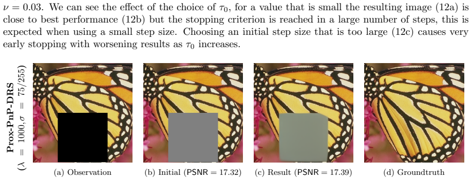
- Large-hole inpainting fails: these Plug-and-Play priors can smooth but cannot hallucinate structured content.
Reading between the lines
- The paper leaves implicit that the hard contraction bound is not certified after training; before trusting the theorems for a deployed Prox-DRUNet, one should measure the spectral norm of $J(\mathrm{Id}-D_\sigma)$ on the image manifold actually visited by the algorithm.
- Because the proximal denoiser differs from the gradient-step denoiser only by the spectral penalty, the natural next step is a hard-Lipschitz architecture that guarantees $L<1$ by construction rather than by soft penalty.
- A testable extension: the explicit potentials $g_\sigma$ and $\varphi_\sigma$ could be differentiated with respect to $\sigma$ and $\lambda$, allowing automatic parameter schedules instead of the current grid tuning.
- The large-hole inpainting failure suggests these priors are local smoothing operators; combining the proximal denoiser with a generative model for hallucination is an obvious extension the paper does not make.
Signed reviews
Editorial analysis
A structured set of objections, weighed in public.
Referee Report
Summary. The paper studies the Gradient-Step Denoiser (GS) and the Proximal Denoiser (Prox) and their use in Plug-and-Play image restoration. It recalls convergence theorems from the authors' prior work [9,10], gives training losses and implementation details for a DRUNet parameterization, and presents experiments on super-resolution, deblurring, and random inpainting. The paper reports that GS-PnP and Prox-PnP algorithms produce explicit objectives F = (1/λ)f + gσ or F = (1/λ)f + φσ, that residuals decay as O(1/√K), and that the parameters σ, λ, and τ0 have interpretable and reproducible effects. It also documents a limitation: these methods cannot perform large-area inpainting because they cannot hallucinate content.
Significance. If the practical claims hold, the paper gives practitioners two convergent Plug-and-Play algorithm families with explicit objective values that can be monitored, which is a meaningful step beyond black-box PnP methods. The recalled theorems are stated accurately, the residual curves are consistent with the announced O(1/√K) rate, and the experiments cover three inverse problems with concrete advice on parameter choices. The use of the public DeepInv library and detailed training prescriptions strengthens reproducibility. The main weakness is that the contraction assumption L<1 (or L<1/2) underpinning the Prox-PnP convergence guarantees is only softly penalized in training and never measured, so the 'convergent' label is conditional on an unverified property of the deployed network.
major comments (3)
- [§3.1, loss (21), and Theorems 3.1–3.3] The convergence guarantees for Prox-PnP require ∇gσ to be L-Lipschitz with L<1 (and L<1/2 for Theorem 3.3), but the training loss (21) only adds a soft penalty µ·max(|||J(Id−Dσ)|||,1−ε) with µ=10⁻³. A soft penalty does not enforce a hard global Lipschitz bound, and the paper reports neither the achieved penalty values, nor the chosen ε, nor any empirical estimate of |||J(Id−Dσ)||| for the trained Prox-DRUNet. Remark 2 merely says it is 'reasonable to assume' Lipschitzness. Therefore the theorems as stated do not apply to the deployed model unless the contraction property is verified; the residual plots in Section 5.2 are consistent with the theory but do not certify the assumption. Please add a direct measurement of the Jacobian spectral norm over the iteration path and test data, or modify the training to enforce a certified hard constraint.
- [§3.3, Theorem 3.3, and §5.2 inpainting] Theorem 3.3 additionally assumes that Im(Dσ) is convex and that L<1/2. The manuscript does not verify either condition for the trained network, and the α=1/2 averaging used for inpainting in Section 5.2 is not connected to the convexity-of-image assumption. Without such verification, the convergence conclusion for Prox-PnP-DRS with nondifferentiable f is not established for the implemented model.
- [§2.4, Algorithm 1, Algorithm 2, Algorithm 4] The backtracking condition in Algorithm 1 appears inverted relative to Section 2.4: Eq. (18) reduces τ when F(x^k)−F(T(x^k)) < (γ/τ)||x^k−T(x^k)||², whereas Algorithm 1 reduces τ when F(x^k)−F(x^{k+1}) ≤ (γ/τ)||x^k−x^{k+1}||². In addition, Algorithm 2 lists z0 and τ0 but never initializes x0, and Algorithm 4 uses Prox_{τf}(z0) without defining τ. These inconsistencies directly affect the reproducibility of the proposed algorithms and should be corrected in a revision.
minor comments (4)
- [§3.2] The name 'Douglas-Rashford Splitting' should be 'Douglas-Rachford Splitting'.
- [§5.2.3] The text says GS-PnP converges for τ < 1/(λ L), but Theorem 2.1 states the condition τ < λ/L; the two should be made consistent.
- [Figure 3 caption] The phrase 'Mean denoising PSNRevolution' should read 'Mean denoising PSNR evolution'.
- [Algorithm 2] The parameter list includes z0 and τ0, but the algorithm body does not use them; add a proper initialization or remove the unused parameters.
Circularity Check
No significant circularity: convergence theorems are transparently imported from prior work by overlapping authors as parameter-free results with explicit assumptions, and the experimental claims are not fitted inputs renamed as predictions.
full rationale
The paper does not derive its convergence guarantees from the training objective; it explicitly recalls them from prior work. Theorem 2.1 and 2.2 are introduced as 'the main theorems established in the paper [9]', and Theorems 3.1–3.3 are presented as results from [10] (e.g., 'Theorem 4.1 in [10]'). Although [9,10] share two co-authors with the present paper, the cited results are stated as parameter-free mathematical theorems with explicit assumptions (L-Lipschitz gradient of gσ, L<1 or L<1/2, boundedness and KL conditions), not as fitted constants, and the present paper tests the induced algorithms on fresh experiments instead of using the theorems to fit the observed curves. The Prox-DRUNet is trained with loss (21), which soft-penalizes the spectral norm of J(Id-Dσ), and no measured Lipschitz constant is reported; thus the convergence guarantee for the deployed network is conditional on an unverified contraction property. This is a correctness or verification gap, not a circularity: the theorem is not equivalent to the training loss by construction, and the paper does not claim the penalty enforces the hard bound. Denoising PSNR on the training objective is reported descriptively and is not used as a predictive test of convergence. Residual decay at the announced O(1/sqrt(K)) rate is observed experimentally and is consistent with the recalled theorems, but consistency of data with a theorem is not a case of the theorem reducing to its inputs. No equation is shown to be identical to another by definition, and no fitted parameter is renamed as a prediction. The self-citations are load-bearing in the sense that the proofs live in [9,10], but those proofs are independent mathematical results with stated assumptions rather than unverified appeals to authority, so the appropriate finding is no significant circularity.
Assumptions & free parameters
free parameters (6)
- lambda (regularization weight) =
0.065 (GS-PnP), 1/0.99 (Prox-PnP), 1000 (large inpainting)
- sigma (denoiser noise level) =
sigma = c*nu with c in {2,3,5} recommended; c up to 10 tested
- tau0 (initial GS-PnP step size) =
tau0 = lambda recommended; 0.1/lambda and 2/lambda tested
- mu (Lipschitz penalty weight) =
1e-3
- beta (DRS averaging parameter) =
not stated
- epsilon in Lipschitz penalty =
not reported
assumptions (6)
- standard math Classical proximal splitting and Kurdyka-Lojasiewicz theory for nonconvex optimization
- domain assumption Observation model y = Ax0 + w with known linear A and white Gaussian noise w
- domain assumption Convolutions use periodic boundary conditions
- ad hoc to paper DRUNet parameterization with ELU or Softplus activations yields differentiable N_sigma with Lipschitz gradient
- ad hoc to paper Soft spectral-norm penalty with power iteration enforces the contraction condition L < 1 or L < 1/2
- domain assumption F is bounded below and iterates are bounded, with coercivity enforced by projection to C = [-1,2]^n
Cite this review
Pith. "Pith review of From the Gradient-Step Denoiser to the Proximal Denoiser and their associated convergent Plug-and-Play algorithms." pith.science (2026). https://pith.science/paper/XBQ52DV3
@misc{pith2026250909793,
  author       = {Pith},
  title        = {Pith review of: From the Gradient-Step Denoiser to the Proximal Denoiser and their associated convergent Plug-and-Play algorithms},
  year         = {2026},
  howpublished = {\url{https://pith.science/paper/XBQ52DV3}},
  note         = {Machine review of arXiv:2509.09793}
}
read the original abstract
In this paper we analyze the Gradient-Step Denoiser and its usage in Plug-and-Play algorithms. The Plug-and-Play paradigm of optimization algorithms uses off the shelf denoisers to replace a proximity operator or a gradient descent operator of an image prior. Usually this image prior is implicit and cannot be expressed, but the Gradient-Step Denoiser is trained to be exactly the gradient descent operator or the proximity operator of an explicit functional while preserving state-of-the-art denoising capabilities.
Figures


Figures from the paper (11 more)


Reference graph
Works this paper leans on
-
[1]
E. Agustsson and R. Timofte , Ntire 2017 challenge on single image super-resolution: Dataset and study , in 2017 IEEE Conference on Computer Vision and Pattern Recognition Workshops (CVPRW), 2017, pp. 1122--1131
work page 2017
-
[2]
H. Attouch, J. Bolte, P. Redont, and A. Soubeyran , Proximal alternating minimization and projection methods for nonconvex problems. an approach based on the kurdyka-lojasiewicz inequality , 2013
work page 2013
-
[3]
Beck , First-Order Methods in Optimization , Society for Industrial and Applied Mathematics, Philadelphia, PA, 2017
A. Beck , First-Order Methods in Optimization , Society for Industrial and Applied Mathematics, Philadelphia, PA, 2017
2017
-
[4]
https://deepinv.github.io/deepinv/
DeepInverse: A deep learning framework for inverse problems in imaging , 2023. https://deepinv.github.io/deepinv/
work page 2023
-
[5]
B. Efron , Tweedie's formula and selection bias , Journal of the American Statistical Association, 106 (2011), pp. 1602--1614
work page 2011
-
[6]
R. Gribonval , Should penalized least squares regression be interpreted as maximum a posteriori estimation? , IEEE Transactions on Signal Processing, 59 (2011), pp. 2405--2410
work page 2011
-
[7]
K. He, X. Zhang, S. Ren, and J. Sun , Deep residual learning for image recognition , 2015
work page 2015
-
[8]
S. Hurault , Convergent plug-and-play methods for image inverse problems with explicit and nonconvex deep regularization , PhD thesis, Universit \'e de Bordeaux, 2023
work page 2023
Show all 28 references
-
[9]
Hurault, A
S. Hurault, A. Leclaire, and N. Papadakis , Gradient step denoiser for convergent plug-and-play , in International Conference on Learning Representations, 2021
2021
-
[10]
height 2pt depth -1.6pt width 23pt, Proximal denoiser for convergent plug-and-play optimization with nonconvex regularization , in International Conference on Machine Learning, 2022
2022
-
[11]
Levin, Y
A. Levin, Y. Weiss, F. Durand, and W. T. Freeman , Understanding and evaluating blind deconvolution algorithms , 2009 IEEE Conference on Computer Vision and Pattern Recognition, (2009), pp. 1964--1971
2009
-
[12]
B. Lim, S. Son, H. Kim, S. Nah, and K. M. Lee , Enhanced deep residual networks for single image super-resolution , 2017
2017
-
[13]
J. Liu, M. S. Asif, B. Wohlberg, and U. S. Kamilov , Recovery analysis for plug-and-play priors using the restricted eigenvalue condition , 2021
2021
-
[14]
K. Ma, Z. Duanmu, Q. Wu, Z. Wang, H. Yong, H. Li, and L. Zhang , Waterloo exploration database: New challenges for image quality assessment models , IEEE Transactions on Image Processing, 26 (2017), pp. 1004--1016
2017
-
[15]
Mallat , A Wavelet Tour of Signal Processing, Third Edition: The Sparse Way , Academic Press, Inc., USA, 3rd ed., 2008
S. Mallat , A Wavelet Tour of Signal Processing, Third Edition: The Sparse Way , Academic Press, Inc., USA, 3rd ed., 2008
2008
-
[16]
Martin, C
D. Martin, C. Fowlkes, D. Tal, and J. Malik , A database of human segmented natural images and its application to evaluating segmentation algorithms and measuring ecological statistics , in IEEE International Conference on Computer Vision. ICCV 2001, vol. 2, 2001, pp. 416--423 vol.2
2001
-
[17]
Pesquet, A
J.-C. Pesquet, A. Repetti, M. Terris, and Y. Wiaux , Learning maximally monotone operators for image recovery , 2021
2021
-
[18]
E. T. Reehorst and P. Schniter , Regularization by denoising: Clarifications and new interpretations , IEEE Transactions on Computational Imaging, 5 (2019), pp. 52--67
2019
-
[19]
Renaud, V
M. Renaud, V. De Bortoli, A. Leclaire, and N. Papadakis , From stability of L angevin diffusion to convergence of proximal MCMC for non-log-concave sampling , arXiv preprint arXiv:2505.14177, (2025)
2025 arXiv
-
[20]
Romano, M
Y. Romano, M. Elad, and P. Milanfar , The little engine that could: Regularization by denoising (red) , 2017
2017
-
[21]
Ronneberger, P
O. Ronneberger, P. Fischer, and T. Brox , U-net: Convolutional networks for biomedical image segmentation , 2015
2015
-
[22]
L. I. Rudin, S. Osher, and E. Fatemi , Nonlinear total variation based noise removal algorithms , Physica D: Nonlinear Phenomena, 60 (1992), pp. 259--268
1992
-
[23]
E. Ryu, J. Liu, S. Wang, X. Chen, Z. Wang, and W. Yin , Plug-and-play methods provably converge with properly trained denoisers , in International Conference on Machine Learning, vol. 97, PMLR, 2019, pp. 5546--5557
2019
-
[24]
Y. Sun, Z. Wu, X. Xu, B. Wohlberg, and U. S. Kamilov , Scalable plug-and-play admm with convergence guarantees , IEEE Transactions on Computational Imaging, 7 (2021), pp. 849--863
2021
-
[25]
A. N. Tikhonov , Solution of incorrectly formulated problems and the regularization method , Soviet Math. Dokl., 4 (1963), pp. 1035--1038
1963
-
[26]
S. V. Venkatakrishnan, C. A. Bouman, and B. Wohlberg , Plug-and-play priors for model based reconstruction , in 2013 IEEE Global Conference on Signal and Information Processing, 2013, pp. 945--948
2013
-
[27]
Zhang, Y
K. Zhang, Y. Li, W. Zuo, L. Zhang, L. V. Gool, and R. Timofte , Plug-and-play image restoration with deep denoiser prior , 2021
2021
-
[28]
N. Zhao, Q. Wei, A. Basarab, N. Dobigeon, D. Kouam \'e , and J.-Y. Tourneret , Fast single image super-resolution using a new analytical solution for _2- _2 problems , IEEE Transactions on Image Processing, 25 (2016), pp. 3683--3697
2016
Reviewed August 15, 2026 · model on record in the stance chip above.
Discussion (0). Continue with ORCID to comment.