REVIEW 4 major objections 5 minor 47 references
Generating Samples of Stationary Distributions of Weakly Interacting Diffusion Models Without Finite Particle Truncation: A Weak Generative Approach
T0 review · 4 major / 5 minor · reviewed 2026-08-04 · deepseek-v4-flash
Pith's one-line read This paper proposes a generative sampler that computes and samples stationary distributions of McKean–Vlasov diffusion processes directly from the weak form of the stationary nonlinear Fokker–Planck equation, with no finite-particle simulat
desk verdict Useful extension of WGS to nonlinear McKean-Vlasov stationary problems with credible low-dimensional results, but the core identifiability of the adaptive Gaussian test-function loss is unproved and the high-dimensional validation leans on the finite-particle simulations the method claims to avoid. read the letter →
The pith
A machine-rendered reading of the paper's core claim, the machinery that carries it, and where it could break.
The reading
What carries the argument
The machinery is the weak form of the stationary nonlinear Fokker-Planck equation, ⟨L*_p φ, p⟩=0 for all smooth test functions φ, together with a normalizing-flow transport map Gθ that pushes a base density to p. In practice the test functions are Gaussians centered at generated samples with width κ, and the loss (18)/(19) evaluates the adjoint operator on these functions using samples from the flow. II-WGS threads the current generative map into the interaction term; PI-WGS holds a frozen approximation of the law in the interaction while updating the map. This combination avoids density derivatives, positivity constraints, and any N-body simulation.
What would settle it
Compare II-WGS/PI-WGS output against a reliable long-time N-particle simulation in a regime where uniform propagation of chaos is known to hold (e.g., the linear Example 1). If the generated samples and the empirical one-particle distribution differ by more than Monte Carlo error (in a chosen metric such as 1-Wasserstein distance), the method is not computing the true stationary law. Alternatively, evaluate the weak residual ⟨L*_p φ_ζ, p̂θ⟩ on a dense grid of Gaussian centers ζ; if the residual is large for some ζ while the empirical loss (14) is small, the test-function family is insufficient
Extended reading notes
Core claim
For a McKean–Vlasov process, invariant measures solve the stationary nonlinear Fokker-Planck equation (SNFPE), a self-consistent PDE because the drift depends on the law through a convolution. The paper discovers that this equation can be turned into a training objective for a normalizing flow: plug transported samples into the adjoint equation, evaluate against Gaussian test functions, and minimize the squared violations. The mean-field interaction is either included implicitly in the loss (II-WGS) or frozen from the previous iterate (PI-WGS). The resulting generative maps produce i.i.d. samples that follow a true stationary measure of the mean-field process, including, with II-WGS, all sta
Load-bearing premise
The load-bearing assumption is that the chosen finite family of Gaussian test functions, with a manually fixed width κ, is rich enough that minimizing the empirical weak loss forces the generated distribution to satisfy the true stationary nonlinear Fokker-Planck equation; this sufficiency is not proved, and the paper only discusses the limits κ→∞ and κ→0.
Editorial extensions
If this is right
- Stationary measures of McKean–Vlasov systems can be sampled as i.i.d. draws directly from the mean-field limit, with no need to simulate N interacting particles.
- In phase-transition regimes, II-WGS can resolve multiple coexisting stationary distributions, including unstable ones that finite-particle simulations typically miss or average over.
- PI-WGS provides a branch-selective alternative that converges to stable stationary solutions, matching the contraction behaviour of fixed-point iterations.
- The method extends to non-gradient drift, parametric interaction kernels, and high-dimensional state spaces, with numerical evidence in 10 and 30 dimensions.
- Conditioning the normalizing flow on a physical parameter (e.g., the colored-noise correlation time) yields a single model that approximates stationary distributions over a range of parameter values, including extrapolation.
Reading between the lines
- Because the weak-loss construction only needs the adjoint of the linearized stationary operator, the same recipe could be applied to other nonlinear stationary PDEs with a transport-map representation, such as Vlasov–Fokker–Planck systems or fractional-diffusion limits.
- The ability of II-WGS to converge to unstable stationary branches suggests it could be used to trace complete bifurcation diagrams for McKean–Vlasov equations, a task where fixed-point and Monte Carlo methods are systematically biased.
- The unresolved gap between the practical Gaussian test-function loss and the exact weak formulation implies that a quantitative guarantee would require either a completeness proof for the test family or an adaptive κ-schedule that provably controls a stationarity residual; this is an open problem the paper does not settle.
- Parametric conditional flows of this type could be combined with continuation or annealing in temperature to detect hysteresis in mean-field phase transitions, a direct extension the paper does not explore.
Editorial analysis
A structured set of objections, weighed in public.
Referee Report
Summary. This paper extends the Weak Generative Sampler (WGS) of Cai et al. to stationary distributions of McKean-Vlasov processes. It proposes two training schemes (II-WGS and PI-WGS) for a normalizing flow: minimize an empirical weak-form residual of the stationary nonlinear Fokker-Planck operator using adaptive Gaussian test functions, with the mean-field convolution evaluated either from current samples (implicit) or from a previous frozen model (Picard). Numerical experiments cover a linear Gaussian test case, a double-well model with phase transition, a parameterized active-particle model, a 10D non-gradient system, and a 30D truncated-Coulombic system. The paper claims the approach is free from finite-particle truncation and can capture all stationary branches when multiple invariant measures exist.
Significance. The problem is important: finite-particle simulation can be unreliable in metastable mean-field systems, and a PDE-based generative sampler would be a useful tool. The weak-form derivation in Section III is standard and clean; the Gaussian example provides a closed-form check; the double-well comparison against a fixed-point iteration is a genuinely external validation that supports the existence of multiple stationary branches; and the parametric active-particle experiment is a nice demonstration of generalization. However, the central identifiability step is unproved, and the high-dimensional validation relies on the very finite-particle simulations the method claims to avoid. These gaps must be addressed before the central claim is supported. If the identifiability gap can be closed, the method would be a significant contribution to computational mean-field models.
major comments (4)
- [Sec. III.A, Eqs. (14)-(15); Sec. III.B, Eqs. (18)-(19)] The empirical loss is a finite projection of the stationary residual onto N_phi Gaussians centered at generated samples. The paper's own discussion of kappa->infinity (loss vanishes) and kappa->0 (strong residual at centers) does not cover the intermediate kappa values used in the experiments. No completeness or identifiability result shows that a small value of this loss implies L_p p is small as a distribution. Moreover, centers are drawn from the current approximate measure, so a wrong density that matches the residual near sampled centers but is arbitrary elsewhere can have small loss. This is load-bearing: the output is claimed to be i.i.d. samples from an invariant measure. Please supply an identifiability/sufficiency result, or a quantitative residual bound, or at least out-of-sample tests on independent test functions not adapted to the current samples.
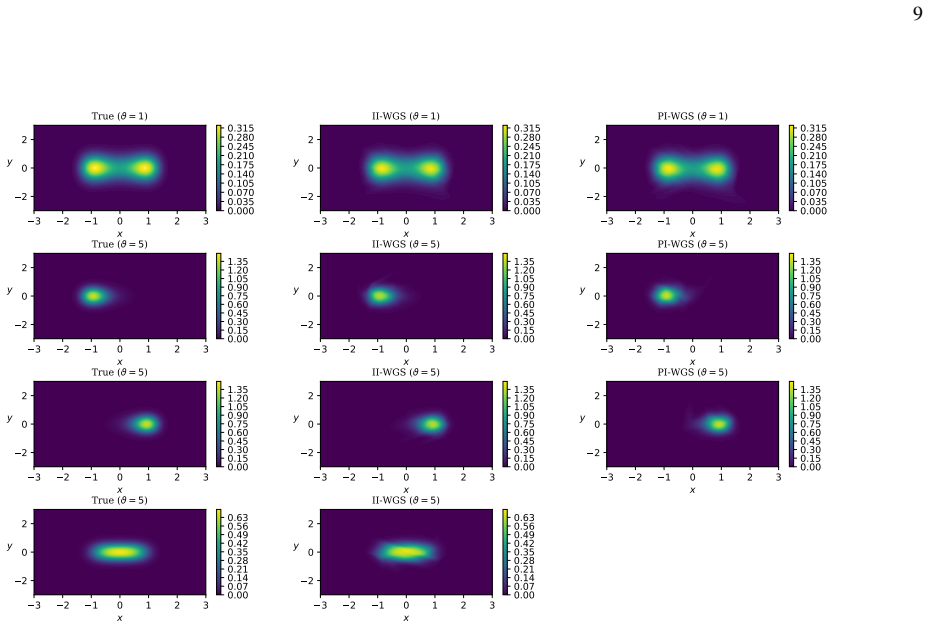
- [Sec. IV.D and Sec. IV.E] The 'true' distributions in the high-dimensional examples are obtained by Euler-Maruyama simulation of N=1000 particles over T=1e5 with burn-in T0=100. This is exactly the finite-particle truncation that the introduction argues can fail for metastable systems (Sec. I). No convergence study in N and T is reported, and no time-uniform propagation of chaos is available for these models. Thus these experiments do not validate the central claim of computing mean-field stationary distributions without finite-particle truncation. The double-well example, validated by fixed-point iteration, is the only external PDE-based check; the high-dimensional examples need a comparable reference or careful N/T convergence analysis.
- [Appendix A, Eqs. (A7)-(A10); Sec. IV.B] The contraction condition beta * theta * Var_{p_bar_x}(x) < 1 is derived for the scalar fixed-point iteration x_{n+1} = F(x_n) in one dimension. This is used to conclude that PI-WGS 'resembles' a non-contractive fixed-point iteration and therefore cannot reach the unstable branch. However, no formal link is established between Algorithm 3 and the gradient-descent training dynamics of the normalizing flow in PI-WGS. The reduction of the 2D Example 2 to two independent 1D marginals is also assumed rather than proved. Please either provide a precise relationship or present the contraction argument as a heuristic explanation rather than a conclusion about PI-WGS.
- [Sec. III.A, Eq. (15)] The ball penalty L_b restricts all generated samples to B_r(x0). For the models considered (linear, quadratic, or harmonic confining potentials), the true stationary measures have unbounded Gaussian tails, so this penalty introduces a truncation bias. The paper does not report r for most experiments or quantify the effect of the truncation. Because L_b can be minimized by concentrating mass inside the ball, it also interacts with the identifiability issue of the weak loss. Please report r for all experiments and provide a sensitivity analysis, or replace L_b with a regularization that is consistent with the decay of the true stationary solution.
minor comments (5)
- [Sec. I, III.A, Algorithm 2] Typos: 'proorogation' (Sec. I), 'avarage' (Sec. III.A), 'generaive' (Algorithm 2 output), 'normalizatoin' (Sec. II.B).
- [Sec. III.A, Eqs. (7)-(13)] The weak form is stated for C_c^infinity test functions, while the implemented Gaussian test functions have unbounded support. This is likely justified by Gaussian decay, but the growth/decay conditions on f, K, and p needed for integration by parts should be stated.
- [Sec. IV] The values of the ball radius r and penalty parameters lambda, c are not reported for Examples 4 and 5. Without these, the experiments are not fully reproducible.
- [Sec. IV.D and IV.E] The high-dimensional examples report only visual histogram comparisons. Quantitative errors such as relative L2 distance or Wasserstein distance are reported only for Examples 1 and 3.
- [Sec. II.A, Eq. (4)] The sum index in the individual potential term is written as n while the sum elsewhere uses i; please standardize the notation.
Circularity Check
No significant circularity: the weak-form derivation is self-contained, self-citation is not load-bearing, and external benchmarks validate the method.
full rationale
The paper's central derivation is the weak-form stationary Fokker-Planck equation (8)-(12), which is exact and not defined in terms of the method's outputs. The loss functions (18) and (19) are direct Monte Carlo approximations of a self-consistent weak residual; no quantity is fitted to a target and then renamed as a prediction. The Gaussian test-function family (13) is an acknowledged ansatz inherited from [CCHZ24], but the paper does not use that citation to prove correctness; it reports numerical validation against an analytical Gaussian solution (Example 1), a fixed-point iteration for the double-well ground truth (Example 2), and SDE simulations in Examples 4-5. Example 3 is a genuine out-of-sample test: training on epsilon in [0.3,0.6] and evaluating on [0.1,0.8]. The Appendix stability condition beta*theta*Var is derived analytically from the fixed-point map, not from the trained model. The self-citation of [CCHZ24] is a methodological precursor, not a load-bearing uniqueness theorem or a substitute for verification. The paper does leave an identifiability gap: it is not proved that the finite, adaptively centered Gaussian test functions are rich enough to force the residual to vanish at intermediate kappa. That is a limitation in the mathematical guarantee, but it is not circular because the loss is not constructed so that its minimizer is the answer by definition. No prediction reduces to an input by construction.
Assumptions & free parameters
free parameters (3)
- Gaussian kernel width kappa =
1.0 (Ex1); 0.3/0.5 (Ex2); 1.0 to 0.8 (Ex3); 1.2 to 0.8 (Ex4); 10 and 11 to decay (Ex5)
- ball penalty radius r and strength lambda, c =
not reported
- center noise scale gamma =
0.8 to 0.08 (Ex5); others unreported
assumptions (4)
- standard math The stationary Fokker-Planck equation (2) is well-posed with the stated boundary and normalization conditions, and its weak form (7) is equivalent to the strong form for C_c^infinity test functions.
- ad hoc to paper A finite family of Gaussian kernels (13), with centers on generated samples and width kappa, suffices to determine the stationary distribution.
- ad hoc to paper The ball constraint Lb does not bias the solution, i.e., all stationary distributions have support inside B_r(x0).
- ad hoc to paper The training dynamics of PI-WGS follow the scalar fixed-point iteration (A7), so the local contraction condition (A10) determines which stationary solution is reached.
Cite this review
Pith. "Pith review of Generating Samples of Stationary Distributions of Weakly Interacting Diffusion Models Without Finite Particle Truncation: A Weak Generative Approach." pith.science (2026). https://pith.science/paper/FGWQAZDV
@misc{pith2026250912841,
  author       = {Pith},
  title        = {Pith review of: Generating Samples of Stationary Distributions of Weakly Interacting Diffusion Models Without Finite Particle Truncation: A Weak Generative Approach},
  year         = {2026},
  howpublished = {\url{https://pith.science/paper/FGWQAZDV}},
  note         = {Machine review of arXiv:2509.12841}
}
read the original abstract
Computing the stationary probability density and generating corresponding samples for the mean-field model of an infinite number of weakly interacting diffusion particles pose significant numerical challenges, particularly in the phase transition regime where the interchangeability of infinite-time and infinite-particle limits breaks down. Traditional approaches, such as direct simulation of finite-particle systems, often fail to accurately pinpoint multiple stationary distributions in the mean-field meta-stable setting. On the other hand, solving the high-dimensional McKean-Vlasov partial differential equation using neural networks typically yields only the density function, limiting its utility for estimating statistical quantities from generating samples. In this work, we propose a novel generative framework based on the weak PDE formulation of the mean-field model to address these challenges. Our approach simultaneously computes the stationary distributions of McKean-Vlasov processes and generates independent and identically distributed samples that satisfy these distributions. This integrated approach not only reveals the true stationary distributions without the random perturbation of finite particle truncation, but also offers deeper insight into the system's behavior in the mean-field limit. Extensive numerical experiments demonstrate the effectiveness of the proposed method, showcasing its ability to accurately approximate stationary distributions, capture intricate phase transitions, and handle high-dimensional complex systems.
Figures


Figures from the paper (7 more)


Reference graph
Works this paper leans on
-
[1]
merlin.mbs aapmrev4-1.bst 2010-07-25 4.21a (PWD, AO, DPC) hacked
FUNCTION id.bst "merlin.mbs aapmrev4-1.bst 2010-07-25 4.21a (PWD, AO, DPC) hacked" ENTRY address archive archivePrefix author bookaddress booktitle chapter collaboration doi edition editor eid eprint howpublished institution isbn issn journal key language month note number organization pages primaryClass publisher school SLACcitation series title translat...
2010
-
[2]
merlin.mbs aipauth4-1.bst 2010-07-25 4.21a (PWD, AO, DPC) hacked
FUNCTION id.bst "merlin.mbs aipauth4-1.bst 2010-07-25 4.21a (PWD, AO, DPC) hacked" ENTRY address archive archivePrefix author bookaddress booktitle chapter collaboration doi edition editor eid eprint howpublished institution isbn issn journal key language month note number organization pages primaryClass publisher school SLACcitation series title translat...
2010
-
[3]
merlin.mbs aipnum4-1.bst 2010-07-25 4.21a (PWD, AO, DPC) hacked
FUNCTION id.bst "merlin.mbs aipnum4-1.bst 2010-07-25 4.21a (PWD, AO, DPC) hacked" ENTRY address archive archivePrefix author bookaddress booktitle chapter collaboration doi edition editor eid eprint howpublished institution isbn issn journal key language month note number organization pages primaryClass publisher school SLACcitation series title translati...
2010
-
[4]
merlin.mbs apsrev4-1.bst 2010-07-25 4.21a (PWD, AO, DPC) hacked
FUNCTION id.bst "merlin.mbs apsrev4-1.bst 2010-07-25 4.21a (PWD, AO, DPC) hacked" ENTRY address archive archivePrefix author bookaddress booktitle chapter collaboration doi edition editor eid eprint howpublished institution isbn issn journal key language month note number organization pages primaryClass publisher school SLACcitation series title translati...
2010
-
[5]
merlin.mbs apsrmp4-1.bst 2010-07-25 4.21a (PWD, AO, DPC) hacked
FUNCTION id.bst "merlin.mbs apsrmp4-1.bst 2010-07-25 4.21a (PWD, AO, DPC) hacked" ENTRY address archive archivePrefix author bookaddress booktitle chapter collaboration doi edition editor eid eprint howpublished institution isbn issn journal key language month note number organization pages primaryClass publisher school SLACcitation series title translati...
2010
-
[6]
Uniform convergence to equilibrium for granular media
Fran c ois Bolley, Ivan Gentil, and Arnaud Guillin. Uniform convergence to equilibrium for granular media. Archive for Rational Mechanics and Analysis , 208:429--445, 2013
2013
-
[7]
Fundamentals of plasma physics
Jos \'e A Bittencourt. Fundamentals of plasma physics . Springer Science & Business Media, 2013
2013
-
[8]
Galactic dynamics
James Binney and Scott Tremaine. Galactic dynamics . Princeton university press, 2011
2011
Show all 47 references
-
[9]
Probability flow solution of the F okker-- P lanck equation
Nicholas M Boffi and Eric Vanden-Eijnden. Probability flow solution of the F okker-- P lanck equation. Machine Learning: Science and Technology , 4(3):035012, 2023
2023
-
[10]
Weak Generative Sampler to Efficiently Sample Invariant Distribution of Stochastic Differential Equation
Zhiqiang Cai, Yu Cao, Yuanfei Huang, and Xiang Zhou. Weak Generative Sampler to Efficiently Sample Invariant Distribution of Stochastic Differential Equation . arXiv preprint arXiv:2405.19256 , 2024
2024 arXiv
-
[11]
Propagation of chaos: A review of models, methods and applications
Louis-Pierre Chaintron and Antoine Diez. Propagation of chaos: A review of models, methods and applications. I . Models and methods . Kinetic and Related Models , 15(6):895--1015, 2022
2022
-
[12]
Propagation of chaos: A review of models, methods and applications
Louis-Pierre Chaintron and Antoine Diez. Propagation of chaos: A review of models, methods and applications. II . Applications . Kinetic and Related Models , 15(6):1017--1173, 2022
2022
-
[13]
Long-time behaviour and phase transitions for the McKean--Vlasov equation on the torus
Jose Antonio Carrillo, Rishabh S Gvalani, Grigorios A Pavliotis, and Andre Schlichting. Long-time behaviour and phase transitions for the McKean--Vlasov equation on the torus . Archive for Rational Mechanics and Analysis , 235(1):635--690, 2020
2020
-
[14]
Kinetic equilibration rates for granular media and related equations: entropy dissipation and mass transportation estimates
Jos \'e A Carrillo, Robert J McCann, and C \'e dric Villani. Kinetic equilibration rates for granular media and related equations: entropy dissipation and mass transportation estimates. Revista Matematica Iberoamericana , 19(3):971--1018, 2003
2003
-
[15]
Donald A. Dawson. Critical dynamics and fluctuations for a mean-field model of cooperative behavior. Journal of Statistical Physics , 31(1):29--85, 1983
1983
-
[16]
u rgen G\
Donald A. Dawson and J\" u rgen G\" a rtner. Large deviations, free energy functional and quasi-potential for a mean field model of interacting diffusions , volume 78. Memoirs of the American Mathematical Society, 1989
1989
-
[17]
Mean field limit for coulomb-type flows
Mitia Duerinckx and Sylvia Serfaty. Mean field limit for coulomb-type flows. Duke Mathematical Journal , 169(15):2887--2935, 2020
2020
-
[18]
Density estimation using Real NVP
Laurent Dinh, Jascha Sohl-Dickstein, and Samy Bengio. Density estimation using Real NVP . In International Conference on Learning Representations , 2017
2017
-
[19]
T.D. Frank. Nonlinear Fokker-Planck Equations: Fundamentals and Applications . Springer Series in Synergetics. Springer Berlin Heidelberg, 2005
2005
-
[20]
Uniform in time propagation of chaos for the 2D vortex model and other singular stochastic systems
Arnaud Guillin, Pierre Le Bris, and Pierre Monmarch \'e . Uniform in time propagation of chaos for the 2D vortex model and other singular stochastic systems . Journal of the European Mathematical Society , pages 1--28, 2024
2024
-
[21]
Uniform Poincar \'e and logarithmic Sobolev inequalities for mean field particle systems
Arnaud Guillin, Wei Liu, Liming Wu, and Chaoen Zhang. Uniform Poincar \'e and logarithmic Sobolev inequalities for mean field particle systems . The Annals of Applied Probability , 32(3):1590--1614, 2022
2022
-
[22]
Mean field limits for interacting diffusions with colored noise: phase transitions and spectral numerical methods
Susana N Gomes, Grigorios A Pavliotis, and Urbain Vaes. Mean field limits for interacting diffusions with colored noise: phase transitions and spectral numerical methods. Multiscale Modeling & Simulation , 18(3):1343--1370, 2020
2020
-
[23]
Gvalani and André Schlichting
Rishabh S. Gvalani and André Schlichting. Barriers of the McKean–Vlasov energy via a mountain pass theorem in the space of probability measures. Journal of Functional Analysis , 279(11):108720, 2020
2020
-
[24]
Score-based physics-informed neural networks for high-dimensional fokker--planck equations
Zheyuan Hu, Zhongqiang Zhang, George E Karniadakis, and Kenji Kawaguchi. Score-based physics-informed neural networks for high-dimensional fokker--planck equations. SIAM Journal on Scientific Computing , 47(3):C680--C705, 2025
2025
-
[25]
A review of the mean field limits for Vlasov equations
Pierre-Emmanuel Jabin. A review of the mean field limits for Vlasov equations . Kinetic and Related models , 7(4):661--711, 2014
2014
-
[26]
The variational formulation of the fokker--planck equation
Richard Jordan, David Kinderlehrer, and Felix Otto. The variational formulation of the fokker--planck equation. SIAM Journal on Mathematical Analysis , 29(1):1--17, 1998
1998
-
[27]
Random batch methods ( RBM ) for interacting particle systems
Shi Jin, Lei Li, and Jian-Guo Liu. Random batch methods ( RBM ) for interacting particle systems. J. Comput. Phys. , 400(108877):108877, January 2020
2020
-
[28]
Foundations of kinetic theory
M Kac. Foundations of kinetic theory. In Proceedings of the Third Berkeley Symposium on Mathematical Statistics and Probability , volume 3, pages 171--197. University of California Press Berkeley, Los Angeles, California, 1956
1956
-
[29]
Counting the number of stationary solutions of partial differential equations via infinite dimensional sampling
Martin Kolodziejczyk, Michela Ottobre, and Gideon Simpson. Counting the number of stationary solutions of partial differential equations via infinite dimensional sampling. Philosophical transactions. Series A, Mathematical, physical, and engineering sciences , 383(2298):202402...
2025
-
[30]
Model for chemotaxis
Evelyn F Keller and Lee A Segel. Model for chemotaxis. Journal of theoretical biology , 30(2):225--234, 1971
1971
-
[31]
Rhythms and turbulence in populations of chemical oscillators
Yoshiki Kuramoto. Rhythms and turbulence in populations of chemical oscillators. Physica A: Statistical Mechanics and its Applications , 106(1-2):128--143, 1981
1981
-
[32]
Computing the invariant distribution of randomly perturbed dynamical systems using deep learning
Bo Lin, Qianxiao Li, and Weiqing Ren. Computing the invariant distribution of randomly perturbed dynamical systems using deep learning. Journal of Scientific Computing , 91(3):77, 2022
2022
-
[33]
Solving Stationary Nonlinear Fokker--Planck Equations via Sampling
Lei Li, Yijia Tang, and Jingtong Zhang. Solving Stationary Nonlinear Fokker--Planck Equations via Sampling . SIAM Journal on Applied Mathematics , 85(1):249--277, 2025
2025
-
[34]
Score-based transport modeling for mean-field Fokker-Planck equations
Jianfeng Lu, Yue Wu, and Yang Xiang. Score-based transport modeling for mean-field Fokker-Planck equations . Journal of Computational Physics , 503:112859, 2024
2024
-
[35]
A random-batch Monte Carlo method for many-body systems with singular kernels
Lei Li, Zhenli Xu, and Yue Zhao. A random-batch Monte Carlo method for many-body systems with singular kernels . SIAM Journal on Scientific Computing , 42(3):A1486--A1509, 2020
2020
-
[36]
Analysis of 1 + 1 dimensional stochastic models of liquid crystal polymer flows
Tiejun Li, Pingwen Zhang, and Xiang Zhou. Analysis of 1 + 1 dimensional stochastic models of liquid crystal polymer flows. Comm. Math. Sci. , 2(2):295--316, 2004
2004
-
[37]
H. P. McKean . A class of markov processes associated with nonlinear parabolic equations. Proceedings of the National Academy of Sciences , 56(6):1907--1911, 1966
1907
-
[38]
H. P. McKean . Propagation of chaos for a class of nonlinear parabolic equations. Lecture Series in Differential Equations , 7:41--57, 1967
1967
-
[39]
Long-time propagation of chaos and exit times for metastable mean-field particle systems
Pierre Monmarch \'e . Long-time propagation of chaos and exit times for metastable mean-field particle systems. arXiv preprint arXiv:2503.00157 , 2025
2025 arXiv
-
[40]
\"O ttinger
H.C. \"O ttinger. Stochastic Processes in Polymeric Fluids: Tools and Examples for Developing Simulation Algorithms . Springer-Verlag, Berlin Heidelberg, 1996
1996
-
[41]
Normalizing flows for probabilistic modeling and inference
George Papamakarios, Eric Nalisnick, Danilo Jimenez Rezende, Shakir Mohamed, and Balaji Lakshminarayanan. Normalizing flows for probabilistic modeling and inference. Journal of Machine Learning Research , 22(57):1--64, 2021
2021
-
[42]
From microscopic to macroscopic scale equations: mean field, hydrodynamic and graph limits
Thierry Paul and Emmanuel Tr \'e lat . From microscopic to macroscopic scale equations: mean field, hydrodynamic and graph limits . arXiv e-prints , page arXiv:2209.08832, September 2022
2022 arXiv
-
[43]
Variational inference with normalizing flows
Danilo Rezende and Shakir Mohamed. Variational inference with normalizing flows. In International conference on machine learning , pages 1530--1538. PMLR, 2015
2015
-
[44]
Entropy-dissipation Informed Neural Network for McKean-Vlasov Type PDEs
Zebang Shen and Zhenfu Wang. Entropy-dissipation Informed Neural Network for McKean-Vlasov Type PDEs . Advances in Neural Information Processing Systems , 36, 2024
2024
-
[45]
Topics in propagation of chaos
Alain-Sol Sznitman. Topics in propagation of chaos. In Paul-Louis Hennequin, editor, Ecole d'Et \'e de Probabilit \'e s de Saint-Flour XIX --- 1989 , volume 1464 of Lecture Notes in Mathematics , pages 165--251. Springer Berlin Heidelberg, 1991
1989
-
[46]
Phase transitions of McKean--Vlasov processes in double-wells landscape
Julian Tugaut. Phase transitions of McKean--Vlasov processes in double-wells landscape . Stochastics An International Journal of Probability and Stochastic Processes , 86(2):257--284, 2014
2014
-
[47]
Adaptive Deep Density Approximation for Fractional Fokker--Planck Equations
Li Zeng, Xiaoliang Wan, and Tao Zhou. Adaptive Deep Density Approximation for Fractional Fokker--Planck Equations . Journal of Scientific Computing , 97(3):68, 2023
2023
Reviewed August 4, 2026 · model on record in the stance chip above.
Discussion (0). Continue with ORCID to comment.