Efficient Sliced Wasserstein Distance Computation via Adaptive Bayesian Optimization

David Hyde; Manish Acharya

REVIEW 4 major objections 3 minor 22 references

Efficient Sliced Wasserstein Distance Computation via Adaptive Bayesian Optimization

T0 review · 4 major / 3 minor · reviewed 2026-08-15 · deepseek-v4-flash

Challenge this review Re-run · record.json Download PDF Read on arXiv ↗ Review JSON

Pith's one-line read Bayesian optimization can select sliced-Wasserstein projection directions that match or beat quasi-Monte Carlo baselines inside optimization loops.

desk verdict First real BO-for-SW direction selector, but the claimed SOTA isn't isolated from simple high-value replacement bias. read the letter →

arxiv 2509.17405 v2 pith:RKA76GQF submitted 2025-09-22 cs.LG

Manish Acharya , David Hyde This is my paper · ORCID

classification cs.LG

keywords slicedWassersteindistanceBayesianoptimizationquasi-MonteCarloprojectiondirectionselectiongradientflowspoint-cloudautoencoderoptimaltransportadaptiveestimation

verification ladder T0 review T1 audit T2 compute T3 formal

The pith

A machine-rendered reading of the paper's core claim, the machinery that carries it, and where it could break.

The reading

The paper argues that when the sliced Wasserstein distance (SW) is evaluated repeatedly inside an optimization loop, fixed direction sets—whether Monte Carlo or quasi-Monte Carlo—ignore information already collected from previous slices. It treats the per-direction cost $f(\theta;\mu,\nu)=W_p^p(\theta_\sharp\mu,\theta_\sharp\nu)$ as a black-box function on the unit sphere and selects directions with Bayesian optimization (BO), yielding four drop-in selectors: BOSW, RBOSW, ABOSW, and ARBOSW. The central empirical claim is that task-adapted directions accelerate or match the best QMC-based estimates in optimization-in-the-loop settings: ARBOSW gives the best final Wasserstein-2 distance in point-cloud interpolation, and ABOSW gives the lowest reconstruction loss in a deep point-cloud autoencoder, both compared against the QSW baseline suite. A sympathetic reader would care because this means SW users can replace or complement QMC direction sets with BO-selected ones without changing downstream losses, gradients, or the option of unbiased randomized estimation.

What carries the argument

The load-bearing object is the slice landscape $f(\theta;\mu,\nu)=W_p^p(\theta_\sharp\mu,\theta_\sharp\nu)$ on the unit sphere $S^{d-1}$. A Gaussian-process surrogate with the angular RBF kernel $k(\theta,\theta')=\exp\bigl(-\tfrac12(d_S(\theta,\theta')/\ell)^2\bigr)$, $d_S(\theta,\theta')=\arccos\langle\theta,\theta'\rangle$, uses a median heuristic for the lengthscale $\ell$; the UCB acquisition $\alpha_t(\theta)=\mu_{t-1}(\theta)+\beta\sigma_{t-1}(\theta)$ with $\beta=0.7$ scores a candidate pool of 4096 uniform directions and proposes batches of five. ABOSW and ARBOSW seed the GP with QSW direction sets and replace the $b$ worst directions after each round, so the machinery converts the SW estimator from a fixed quadrature rule into an adaptive selector that exploits feedback from previously evaluated slices.

What would settle it

Construct point clouds whose slice function $f(\theta;\mu,\nu)$ is effectively supported only in a narrow cap of angular radius well below the median pairwise spacing of the QSW seed; if, across many trials, BO-refined sets (ABOSW/ARBOSW) do not match or beat the unrefined QSW seed in the point-cloud interpolation task, the smoothness-informativeness premise fails.

Watch

Extended reading notes

Core claim

The paper's central discovery is empirical: a small set of BO-refined projection directions, seeded from QSW direction sets, can reach the best reported convergence for SW-based optimization loops. Concretely, ARBOSW achieves a final Wasserstein-2 distance of $0.003 \pm 0.000$ at step 500 in point-cloud interpolation (same mean as the best randomized QSW variants, with smaller variance), and ABOSW achieves the lowest reconstruction loss in the deep point-cloud autoencoder task ($\mathrm{SW}_2 = 1.81 \pm 0.02$ versus $1.84 \pm 0.02$ for CQSW at epoch 400). The paper also establishes the boundary of the claim: on one-shot approximation of the spherical integral, BOSW trails both MC and QSW, so the advantage is specific to settings where SW appears inside an optimization loop and the direction set can be adapted to the task.

Load-bearing premise

The method assumes the slice function $f(\theta)=W_p^p(\theta_\sharp\mu,\theta_\sharp\nu)$ is smooth enough on the sphere that a Gaussian-process surrogate with an angular RBF kernel and median lengthscale produces informative UCB proposals; if $f$ varies at scales below that lengthscale, the selected directions are no more useful than random or QMC ones.

Editorial extensions

If this is right

QSW direction sets can serve as a seed rather than a finished design: a few BO refinement rounds improve optimization-in-the-loop performance with modest runtime overhead (ARBOSW at roughly 7 s versus 4–4.3 s for QSW baselines in the interpolation task).
SW-based gradient flows and deep autoencoder training can adopt BO selectors without touching the downstream loss, the gradient computation, or the unbiasedness option provided by RQSW-style randomization.
The optimal direction strategy is task-dependent: stable large datasets favor one-shot or seeded hybrids (BOSW/ABOSW), while evolving flows favor refresh or restart hybrids (RBOSW/ARBOSW).
The Appendix D asymptotic note implies the advantage of BOSW is finite-$L$: with constant UCB $\beta$ the selector would converge toward the supremum of $f$, not its uniform average, so long-run unbiased estimation requires annealing $\beta$ or switching to MC/RQSW.

Reading between the lines

Editorial extensions of the paper, not claims the author makes directly.

The same selector machinery could be applied to other families of slice-based divergences (generalized sliced Wasserstein, max-sliced variants) because it only requires a scalar per-direction cost; the paper does not make this extension.
A cheap diagnostic for why ABOSW/ARBOSW help would be to record which seed directions get replaced during refinement; if only the lowest-value slices are swapped out, the gain comes from pruning bad directions rather than from global landscape learning.
The paper's appeal to high-dimensional BO results suggests a concrete testable extension: run ARBOSW on point clouds in dimension $d\ge 32$ with the same angular RBF kernel, and check whether the median-lengthscale heuristic still yields informative proposals.
The task-dependence of the best variant implies that SW libraries could expose direction selection as a plug-in choice rather than hard-coding QMC, an interface the paper does not propose.

Share X Bluesky LinkedIn Reddit HN

Signed reviews

No signed human review yet.

Editorial analysis

A structured set of objections, weighed in public.

Desk editor's note, referee report, and a circularity audit.

Desk Editor's Note

read the letter

Here's the short version: this is the first application of Bayesian optimization to SW direction selection I'm aware of, and the QSW-seeded hybrid is a new idea. The paper is worth engaging, but the 'state-of-the-art' headline is not yet supported. The main missing experiment is a control that spends the same refinement budget without the GP surrogate.

What's good: the method family is clearly described and genuinely drop-in. The authors are honest where things fail: BOSW is bad on approximation error, RGQSW beats them on style transfer, and Appendix D concedes UCB selects toward sup f with no finite-L bound. The ablations on acquisition function, beta, cosine cutoff, and pool size are real work, and the citation pattern looks fair.

The load-bearing problem: ABOSW replaces worst QSW directions with UCB proposals, but there is no control that randomly replaces worst directions or brute-force picks the highest-f candidates from the same pool. The gains in Tables 1 and 2 may simply come from swapping low-value directions for high-value ones; the GP's modeling of the slice landscape is never isolated. Appendix D makes this more than a quibble: with constant beta, UCB is biased by design. The numbers are also marginal: ARBOSW ties REQSW/RCQSW at step 500, and ABOSW beats CQSW by 0.03 in SW2 with overlapping spread. Hyperparameters were tuned on the Section 4.3 task, which is also a main result, so some of the advantage is selected. Section 4.1 is a BO showcase against static integration rules rather than a fair SW baseline. No code is released.

Who gains: practitioners using SW inside optimization loops who want a clear, adaptive direction selector and an honest map of its strengths. The paper should go to review, but only with the expectation of a revision: add control experiments, untuned results, code, and toned-down claims.

Referee Report

4 major / 3 minor

Summary. The paper proposes four Bayesian-optimization-based selectors (BOSW, RBOSW, ABOSW, ARBOSW) for the projection directions used in estimating sliced Wasserstein distances, and evaluates them on approximation error, point-cloud interpolation, image style transfer, and deep point-cloud autoencoder training, following the QSW benchmark protocol of Nguyen et al. The central claim is that these selectors achieve state-of-the-art convergence in optimization-in-the-loop settings, particularly in gradient flows and autoencoder training.

Significance. The idea of using BO for SW direction selection is novel (per the cited survey) and the drop-in design is clean and potentially useful. The authors are transparent in their appendices, acknowledging the bias of UCB toward sup f, the superior performance of RGQSW on style transfer, and the tuning of hyperparameters on the point-cloud interpolation task. However, the experimental support for the headline claim is thin: the reported gains are small, often within noise, and no control experiment isolates the effect of the GP surrogate. If the results are reproduced with proper controls, the contribution is a modest but interesting extension of the SW toolbox.

major comments (4)

[§4.3 Table 1; §4.5 Table 2] The abstract and conclusion claim that the proposed methods 'achieve state-of-the-art performance' and 'state-of-the-art convergence' for point-cloud interpolation and deep autoencoder tasks. The reported numbers do not support this. In Table 1 at step 500, ARBOSW is 0.003±0.000, statistically indistinguishable from REQSW and RCQSW at 0.003±0.001, and RBOSW (0.018) is clearly worse. In Table 2, the best BO variant is BOSW at SW2=1.80±0.01, only slightly below CQSW at 1.84±0.02 with overlapping error bars, and the text's identification of ABOSW as the best is contradicted by the table, where BOSW has the lower value. No significance testing is reported, and three-seed means do not establish superiority.
[Appendix A.2, Figures 5-6] The image style transfer experiment contradicts the claim that BO hybrids are competitive with the state of the art. At L=100, RGQSW reaches W2=0.12 while ARBOSW reaches 0.65 and ABOSW 18.50; at L=10, RGQSW reaches 1.25 vs ARBOSW 1.37. The main text acknowledges this but describes RGQSW as 'marginally stronger,' which understates a factor-of-five gap. Since style transfer is one of the three core optimization-in-the-loop tasks, this is directly relevant to the central claim and weakens it.
[§3.2, §4.1, Appendix D] There is no control experiment that attributes the observed convergence gains to Bayesian optimization itself. ABOSW changes at most 10 of 100 directions (r=2, b=5) by replacing the worst directions with UCB proposals, and ARBOSW repeats this; a random-replacement control or a brute-force highest-f replacement control would use the same budget. Appendix D explicitly notes that UCB with constant beta=0.7 drives the estimator toward sup f, so the gains could simply reflect high-f bias rather than the GP surrogate's modeling ability. Without such a control, the paper's causal claim about BO is untested.
[Appendix C] All hyperparameters (acquisition function, beta, cosine cutoff, nc) were selected by ablations on the point-cloud interpolation task of Section 4.3, and Table 1 reports results on that same task. This self-confirming tuning means the interpolation results cannot serve as unbiased evidence for the method. The paper should either tune on a separate validation task or demonstrate robustness across hyperparameter choices on held-out tasks.

minor comments (3)

[§4.2, Figure 2] The approximation error plot includes only BOSW, not RBOSW/ABOSW/ARBOSW; adding a sentence in the text or caption explaining this omission would prevent confusion, since the hybrids are claimed to be drop-in selectors.
[§3.1, Eq. (3)] The kernel uses geodesic distance dS(θ,θ') = arccos⟨θ,θ'⟩, while near-duplicates are suppressed by cosine similarity > 0.98. Please clarify whether the GP is fit after duplicate suppression and whether the candidate pool is sampled uniformly on S^{d-1} independently at each round.
[Table 2] The caption states 'Losses are scaled by 10^2 for ease of exposition,' but the table header lists 'SW2(↓) W2(↓)' without indicating the scaling; standardizing the notation and making the scaling explicit in the header would improve readability.

Circularity Check

0 steps flagged · score 2.0 of 10

No derivation reduces to its inputs; the only mild self-confirming element is that BO hyperparameters were selected on the same point-cloud interpolation benchmark later used for the headline SOTA claim.

full rationale

The paper's claims are empirical rather than deductive, and no equation or fitted parameter is renamed as a prediction. The objective f(theta;mu,nu)=W_p^p(theta#mu,theta#nu), the GP angular-RBF surrogate, and the UCB acquisition are defined independently of the downstream accuracy results, and the QSW baselines are external prior work. Appendix D is transparent that the BO-MC error term is unproved and that constant-beta UCB is biased toward sup f, so the reported state-of-the-art performance is presented as experimental evidence, not as a consequence of the definitions. The one self-confirming element is that Section 3.1 states 'We performed ablations to choose the models and parameters listed here; see Appendix C,' while Appendix C says each ablation 'is evaluated on the point-cloud interpolation (gradient flow) example of Section 4.3'—the same task that produces Table 1. This is a benchmark-tuning concern on one experiment, not a logical circularity: the autoencoder result in Table 2 is a separate task, and the incidental citation of Vardhan et al. (2024), which shares an author, is not load-bearing. Overall, the central derivation is self-contained, so the circularity score is low.

Assumptions & free parameters 6 free parameters · 4 assumptions · 0 invented entities

The ledger captures hyperparameters tuned on the reported benchmark, a missing refresh period, and the smoothness assumption that underpins the method. No new physical or mathematical entities are postulated.

free parameters (6)

UCB exploration weight beta = 0.7
Chosen via ablation on the point-cloud interpolation task (Appendix C, Fig. 9); not derived.
Cosine similarity cutoff = 0.98
Selected via ablation on point-cloud interpolation (Appendix C, Fig. 10).
Candidate pool size n_c = 4096
Set to match QSW; ablation shows 1024 better for BOSW (Appendix C, Fig. 11).
Mini-batch size b = 5
Stated in Section 3.1; no ablation reported.
Refinement rounds r = 2
Stated in Section 3.2 for ABOSW; no ablation reported.
Refresh period R for RBOSW/ARBOSW = not reported
The paper says 'periodic' but does not specify the interval; a central hyperparameter of the restarted variants.

assumptions (4)

domain assumption The slice landscape f(theta) is smooth enough for a GP with angular RBF kernel to be a useful surrogate.
Invoked in Section 3.1 via Eq. 3; the entire BO selection relies on this.
domain assumption Replacing the current worst directions with UCB proposals improves the SW-based optimization.
Used in ABOSW/ARBOSW (Section 3.2); no proof provided.
domain assumption SW distance is a reliable proxy for the true Wasserstein distance in the outer-loop optimization tasks.
All experiments evaluate W2 and SW2 of the interpolated or trained objects.
standard math The Borel-Cantelli lemma applies to the annealed sampling scheme in Appendix D.
Appendix D invokes it informally to argue eventual uniform coverage, but notes that independence does not hold.

how reviews work

0 comments

Cite this review

Pith. "Pith review of Efficient Sliced Wasserstein Distance Computation via Adaptive Bayesian Optimization." pith.science (2026). https://pith.science/paper/RKA76GQF

@misc{pith2026250917405,
  author       = {Pith},
  title        = {Pith review of: Efficient Sliced Wasserstein Distance Computation via Adaptive Bayesian Optimization},
  year         = {2026},
  howpublished = {\url{https://pith.science/paper/RKA76GQF}},
  note         = {Machine review of arXiv:2509.17405}
}

abstract

The sliced Wasserstein distance (SW) reduces optimal transport on $\mathbb{R}^d$ to a sum of one-dimensional projections, and thanks to this efficiency, it is widely used in geometry, generative modeling, and registration tasks. Recent work shows that quasi-Monte Carlo constructions for computing SW (QSW) yield direction sets with excellent approximation error. This paper presents an alternate, novel approach: learning directions with Bayesian optimization (BO), particularly in settings where SW appears inside an optimization loop (e.g., gradient flows). We introduce a family of drop-in selectors for projection directions: BOSW, a one-shot BO scheme on the unit sphere; RBOSW, a periodic-refresh variant; ABOSW, an adaptive hybrid that seeds from competitive QSW sets and performs a few lightweight BO refinements; and ARBOSW, a restarted hybrid that periodically relearns directions during optimization. Our BO approaches can be composed with QSW and its variants (demonstrated by ABOSW/ARBOSW) and require no changes to downstream losses or gradients. We provide numerical experiments where our methods achieve state-of-the-art performance, and on the experimental suite of the original QSW paper, we find that ABOSW and ARBOSW can achieve convergence comparable to the best QSW variants with modest runtime overhead.

Figures

Figures reproduced from arXiv: 2509.17405 by the authors.

**Figure 2.** Approximation error for SW between empirical distributions over point clouds. BO does [PITH_FULL_IMAGE:figures/full_fig_p006_2.png] view at source ↗

**Figure 3.** Image style transfer with L=100 and 1,000 iterations. 4.5 DEEP POINT-CLOUD AUTOENCODER Setting. Following Nguyen et al. (2023a) and Nguyen et al. (2024a), we train deep point-cloud autoencoders with SW on ShapeNet Core-55 (Chang et al., 2015). This amounts to optimizing an objective function: min ϕ,ψ EX∼µ(X) [PITH_FULL_IMAGE:figures/full_fig_p008_3.png] view at source ↗

Figures from the paper (8 more)

**Figure 4.** Figure 4: Reconstructed point clouds from the deep autoen [PITH_FULL_IMAGE:figures/full_fig_p009_4.png]

**Figure 5.** Figure 5: Full comparison for image style transfer with [PITH_FULL_IMAGE:figures/full_fig_p015_5.png]

**Figure 6.** Figure 6: Full comparison for image style transfer with [PITH_FULL_IMAGE:figures/full_fig_p015_6.png]

**Figure 7.** Figure 7: Full reconstructed point-clouds from SW, QSW, RQSW, and BO variants with L = 100. [PITH_FULL_IMAGE:figures/full_fig_p016_7.png]

**Figure 8.** Figure 8: Ablation study of different acquisition functions for Bayesian optimization, including [PITH_FULL_IMAGE:figures/full_fig_p017_8.png]

**Figure 9.** Figure 9: Ablation study of different values of β (the weight parameter for the UCB acquisition function). Although the different values of β yield similar results, β = 0.7 consistently demonstrates the best performance. that LCB (identical to UCB, but for minimization rather th…

**Figure 10.** Figure 10: Ablation study of different values of the cosine-similarity cutoff threshold used in our [PITH_FULL_IMAGE:figures/full_fig_p018_10.png]

**Figure 11.** Figure 11: Effect of varying nc on the convergence of our BO-based methods. For most methods, nc = 4096 is optimal, except for BOSW, which attains minimal error after 500 steps using nc = 1024. Note that the vertical axis is scaled logarithmically to make the data points easier…

Review history (2 revisions) →

Discussion (0). Continue with ORCID to comment.

Reference graph

Works this paper leans on

22 extracted references · 11 canonical work pages

[1]

E USE OFLARGELANGUAGEMODELS Large language models (LLMs) were used in the preparation of this paper

It follows that the bias will match that of uniform MC sampling, which is 0 in the limit; and under this scheme, the convergence rate would reachO(L−1/2)asymptotically (whether it is faster or slower during initial iterations). E USE OFLARGELANGUAGEMODELS Large language models (LLMs) were used in the preparation of this paper. Specifically, Perplexity was...

work page 2008
[7]

Deep learning for bayesian optimization of scientific problems with high-dimensional structure.arXiv preprint arXiv:2104.11667,

Samuel Kim, Peter Y Lu, Charlotte Loh, Jamie Smith, Jasper Snoek, and Marin Solja ˇci´c. Deep learning for bayesian optimization of scientific problems with high-dimensional structure.arXiv preprint arXiv:2104.11667,

arXiv
[8]

Gpflowopt: A bayesian optimization library using tensorflow.arXiv preprint arXiv:1711.03845,

Nicolas Knudde, Joachim van der Herten, Tom Dhaene, and Ivo Couckuyt. Gpflowopt: A bayesian optimization library using tensorflow.arXiv preprint arXiv:1711.03845,

arXiv
[9]

Sliced-Wasserstein Estimation with Spherical Harmonics as Control Variates

URLhttps:// arxiv.org/abs/2402.01493. Mark McLeod, Stephen Roberts, and Michael A Osborne. Optimization, fast and slow: optimally switching between local and bayesian optimization. InInternational Conference on Machine Learning, pp. 3443–3452. PMLR,

work page Pith review arXiv
[10]

11 Efficient Sliced Wasserstein Distance Computation via Adaptive Bayesian Optimization Khai Nguyen, Tongzheng Ren, and Nhat Ho

URLhttps: //arxiv.org/abs/2305.00402. 11 Efficient Sliced Wasserstein Distance Computation via Adaptive Bayesian Optimization Khai Nguyen, Tongzheng Ren, and Nhat Ho. Markovian sliced wasserstein distances: beyond inde- pendent projections. InProceedings of the 37th International Conference on Neural Information Processing Systems, NIPS ’23, Red Hook, NY ...

arXiv
[15]

Jasper Snoek, Hugo Larochelle, and Ryan P

URLhttps://arxiv.org/abs/2502.02275. Jasper Snoek, Hugo Larochelle, and Ryan P. Adams. Practical Bayesian optimization of machine learning algorithms. InAdvances in Neural Information Processing Systems (NeurIPS), vol- ume 25,

arXiv
[16]

Constrained bayesian optimization for automatic underwater vehicle hull design

12 Acharya and Hyde Harsh Vardhan, Peter V olgyesi, Will Hedgecock, and Janos Sztipanovits. Constrained bayesian optimization for automatic underwater vehicle hull design. InProceedings of Cyber-Physical Systems and Internet of Things Week 2023, pp. 116–121

work page 2023
[17]

C´edric Villani et al.Optimal transport: old and new, volume

doi: 10.1016/j.oceaneng.2024.118777. C´edric Villani et al.Optimal transport: old and new, volume

arXiv 2024

Show all 22 references

[18]

3d shapenets: A deep representation for volumetric shapes

Zhirong Wu, Shuran Song, Aditya Khosla, Fisher Yu, Linguang Zhang, Xiao Tang, and Jianxiong Xiao. 3d shapenets: A deep representation for volumetric shapes. InProceedings of the IEEE conference on computer vision and pattern recognition, pp. 1912–1920,

1912
[21]

Bounding the performance of BOSW for finiteLis an interesting open question

This rough sketch demonstrates that BOSW, at least with UCB with a constantβ, will not converge in the limit—despite its attractive numerical perfor- mance (demonstrated in our experiments in the main body) during early iterations. Bounding the performance of BOSW for finiteLi...

2021
[100]

Figure 10: Ablation study of different values of the cosine-similarity cutoff threshold used in our method

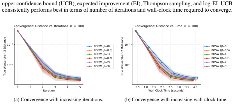
BOSW (cos=0.7) BOSW (cos=0.8) BOSW (cos=0.9) BOSW (cos=0.95) BOSW (cos=0.98) BOSW (cos=1.0) (b) Convergence with increasing wall-clock time. Figure 10: Ablation study of different values of the cosine-similarity cutoff threshold used in our method. The plots motivate our usage...
[1992]

9781611970081

doi: 10.1137/1. 9781611970081. Michael A. Osborne, David Duvenaud, Roman Garnett, Carl E. Rasmussen, Stephen J. Roberts, and Zoubin Ghahramani. Active learning of model evidence using bayesian quadrature. InProceed- ings of the 26th International Conference on Neural Informati...

doi
[2008]

doi: https://doi.org/10.1016/j.spl

ISSN 0167-7152. doi: https://doi.org/10.1016/j.spl. 2007.07.023. URLhttps://www.sciencedirect.com/science/article/pii/ S0167715207002520. Angel X Chang, Thomas Funkhouser, Leonidas Guibas, Pat Hanrahan, Qixing Huang, Zimo Li, Silvio Savarese, Manolis Savva, Shuran Song, Hao Su...

2007 arXiv
[2010]

David Duvenaud

doi: 10.1017/CBO9780511921571. David Duvenaud. Bayesian Quadrature: Model-based Approximate Integration.https:// www.cs.toronto.edu/˜duvenaud/talks/intro_bq.pdf,

doi
[2012]

David Eriksson and Matthias Poloczek

[Online; accessed 21 September 2025]. David Eriksson and Matthias Poloczek. Scalable constrained bayesian optimization. InInternational conference on artificial intelligence and statistics, pp. 730–738. PMLR,

2025
[2015]

Nicolas Bonnotte.Unidimensional and evolution methods for optimal transportation

doi: 10.1007/s10851-014-0506-3. Nicolas Bonnotte.Unidimensional and evolution methods for optimal transportation. PhD thesis, Universit´e Paris Sud-Paris XI; Scuola normale superiore (Pise, Italie),

doi
[2016]

Yihang Shen and Carl Kingsford

doi: 10.1109/JPROC.2015.2494218. Yihang Shen and Carl Kingsford. Computationally efficient high-dimensional bayesian optimization via variable selection.arXiv preprint arXiv:2109.09264,

2015
[2019]

Charles R Qi, Hao Su, Kaichun Mo, and Leonidas J Guibas

doi: 10.1561/2200000073. Charles R Qi, Hao Su, Kaichun Mo, and Leonidas J Guibas. Pointnet: Deep learning on point sets for 3d classification and segmentation. InProceedings of the IEEE conference on computer vision and pattern recognition, pp. 652–660,

doi
[2021]

Nicolas Bonneel, Julien Rabin, Gabriel Peyr ´e, and Hanspeter Pfister

URLhttps://arxiv.org/abs/2004.11324. Nicolas Bonneel, Julien Rabin, Gabriel Peyr ´e, and Hanspeter Pfister. Sliced and radon wasserstein barycenters of measures.Journal of Mathematical Imaging and Vision, 51(1):22–45,

2004 arXiv
[2023]

C ABLATIONSTUDIES Section 3.1 describes several modeling and parameter choices made for our implementation of Bayesian optimization

equipped with an Apple M3 Max chip and 36 GB memory. C ABLATIONSTUDIES Section 3.1 describes several modeling and parameter choices made for our implementation of Bayesian optimization. We justify these choices here via ablation studies. Each study is evalu- ated on the point-...

1933
[2024]

No´emie Jaquier and Leonel Rozo

URLhttps://arxiv.org/abs/2402.02229. No´emie Jaquier and Leonel Rozo. High-dimensional bayesian optimization via nested riemannian manifolds.Advances in Neural Information Processing Systems, 33:20939–20951,

arXiv
[2025]

Gabriel Peyr´e and Marco Cuturi.Computational Optimal Transport, volume 11 ofFoundations and Trends in Machine Learning

URLhttps://arxiv.org/abs/2509.10166. Gabriel Peyr´e and Marco Cuturi.Computational Optimal Transport, volume 11 ofFoundations and Trends in Machine Learning. Now Publishers,

Pith tools

Reviewed August 15, 2026 · model on record in the stance chip above.

[1] [1]

E USE OFLARGELANGUAGEMODELS Large language models (LLMs) were used in the preparation of this paper

It follows that the bias will match that of uniform MC sampling, which is 0 in the limit; and under this scheme, the convergence rate would reachO(L−1/2)asymptotically (whether it is faster or slower during initial iterations). E USE OFLARGELANGUAGEMODELS Large language models (LLMs) were used in the preparation of this paper. Specifically, Perplexity was...

work page 2008

[2] [7]

Deep learning for bayesian optimization of scientific problems with high-dimensional structure.arXiv preprint arXiv:2104.11667,

Samuel Kim, Peter Y Lu, Charlotte Loh, Jamie Smith, Jasper Snoek, and Marin Solja ˇci´c. Deep learning for bayesian optimization of scientific problems with high-dimensional structure.arXiv preprint arXiv:2104.11667,

arXiv

[3] [8]

Gpflowopt: A bayesian optimization library using tensorflow.arXiv preprint arXiv:1711.03845,

Nicolas Knudde, Joachim van der Herten, Tom Dhaene, and Ivo Couckuyt. Gpflowopt: A bayesian optimization library using tensorflow.arXiv preprint arXiv:1711.03845,

arXiv

[4] [9]

Sliced-Wasserstein Estimation with Spherical Harmonics as Control Variates

URLhttps:// arxiv.org/abs/2402.01493. Mark McLeod, Stephen Roberts, and Michael A Osborne. Optimization, fast and slow: optimally switching between local and bayesian optimization. InInternational Conference on Machine Learning, pp. 3443–3452. PMLR,

work page Pith review arXiv

[5] [10]

11 Efficient Sliced Wasserstein Distance Computation via Adaptive Bayesian Optimization Khai Nguyen, Tongzheng Ren, and Nhat Ho

URLhttps: //arxiv.org/abs/2305.00402. 11 Efficient Sliced Wasserstein Distance Computation via Adaptive Bayesian Optimization Khai Nguyen, Tongzheng Ren, and Nhat Ho. Markovian sliced wasserstein distances: beyond inde- pendent projections. InProceedings of the 37th International Conference on Neural Information Processing Systems, NIPS ’23, Red Hook, NY ...

arXiv

[6] [15]

Jasper Snoek, Hugo Larochelle, and Ryan P

URLhttps://arxiv.org/abs/2502.02275. Jasper Snoek, Hugo Larochelle, and Ryan P. Adams. Practical Bayesian optimization of machine learning algorithms. InAdvances in Neural Information Processing Systems (NeurIPS), vol- ume 25,

arXiv

[7] [16]

Constrained bayesian optimization for automatic underwater vehicle hull design

12 Acharya and Hyde Harsh Vardhan, Peter V olgyesi, Will Hedgecock, and Janos Sztipanovits. Constrained bayesian optimization for automatic underwater vehicle hull design. InProceedings of Cyber-Physical Systems and Internet of Things Week 2023, pp. 116–121

work page 2023

[8] [17]

C´edric Villani et al.Optimal transport: old and new, volume

doi: 10.1016/j.oceaneng.2024.118777. C´edric Villani et al.Optimal transport: old and new, volume

arXiv 2024