pith. sign in

arxiv: 2509.22017 · v4 · submitted 2025-09-26 · 💻 cs.LG

AEGIS: Authentic Edge Growth In Sparsity for Link Prediction in Edge-Sparse Bipartite Knowledge Graphs

Pith reviewed 2026-05-18 13:48 UTC · model grok-4.3

classification 💻 cs.LG
keywords link predictionbipartite graphsedge augmentationsparsityknowledge graphsresamplingsemantic augmentationauthenticity
0
0 comments X

The pith

Authenticity-constrained resampling of existing edges matches or improves link prediction in edge-sparse bipartite knowledge graphs.

A machine-rendered reading of the paper's core claim, the machinery that carries it, and where it could break.

The paper introduces AEGIS, a framework that augments training data for link prediction by resampling existing edges in bipartite knowledge graphs instead of fabricating new nodes or edges. It preserves the original node set and tests this on both naturally sparse graphs and denser graphs made sparse through percolation. Evaluations use AUC-ROC and Brier score with statistical tests, showing copy-based variants hold steady while semantic methods add gains when node text is informative. A reader would care because many real niche-domain graphs lack sufficient links, and this offers a data-efficient way to strengthen predictions without introducing inauthentic structure.

Core claim

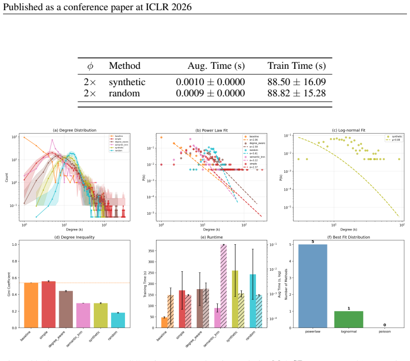
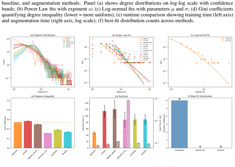
AEGIS is an edge-only augmentation framework that resamples existing training edges, either uniformly or with inverse-degree bias, thereby preserving the original node set and sidestepping fabricated endpoints. On Amazon and MovieLens with induced sparsity, copy-based variants match the sparse baseline while semantic KNN is the only method that restores AUC and calibration; random and synthetic edges remain detrimental. On the text-rich GDP graph, semantic KNN achieves the largest AUC improvement and Brier score reduction, and simple resampling also lowers the Brier score relative to the sparse control.

What carries the argument

AEGIS (Authentic Edge Growth In Sparsity), an edge-only augmentation framework that resamples existing training edges to grow the graph while preserving the original node set and avoiding fabricated endpoints.

If this is right

  • Copy-based AEGIS variants match the sparse baseline on induced-sparse Amazon and MovieLens while semantic KNN restores both AUC and calibration.
  • Random and synthetic edge additions remain detrimental to performance across the tested regimes.
  • On naturally sparse text-rich graphs, semantic KNN yields the largest gains in AUC and Brier score, with simple resampling improving calibration.
  • Authenticity-constrained resampling serves as a data-efficient strategy for sparse bipartite link prediction when node descriptions enable semantic augmentation.

Where Pith is reading between the lines

These are editorial extensions of the paper, not claims the author makes directly.

  • The method could be applied to non-bipartite graphs if the core resampling rule is kept to avoid new nodes.
  • When node descriptions are absent, the uniform or degree-aware copy variants may still provide calibration benefits in sparse settings.
  • Combining AEGIS resampling with different base link predictors might produce additive gains beyond the tested setups.

Load-bearing premise

Inducing sparsity via high-rate bond percolation on denser graphs produces regimes comparable to naturally sparse graphs for evaluating authenticity.

What would settle it

If AEGIS variants fail to match or exceed the sparse baseline on both AUC-ROC and Brier score when tested on additional naturally sparse bipartite graphs without semantic node text, the claim that authenticity-constrained resampling is data-efficient would be falsified.

Figures

Figures reproduced from arXiv: 2509.22017 by Hugh Xuechen Liu, K{\i}van\c{c} Tatar.

Figure 1
Figure 1. Figure 1: Amazon (product–category), GAT, q=0.01, ϕ=100: Comprehensive degree analysis (M ± SD, n = 32 seeds). Panel (a) shows degree distributions on log-log scale with ±1σ confidence bands; (b) Power Law fits with exponent α (lower α = heavier tail); (c) Log-normal fits with parameters µ and σ; (d) Gini coefficients quantifying degree inequality (0=perfect equality, 1=maximum inequality); (e) best-fit distribution… view at source ↗
Figure 2
Figure 2. Figure 2: MovieLens (movie–genre), GAT, q=0.01, ϕ=100: Comprehensive degree analysis (M±SD, n = 32 seeds). Panel (a) shows degree distributions on log-log scale with ±1σ confidence bands; (b) Power Law fits with exponent α (lower α = heavier tail); (c) Log-normal fits with parameters µ and σ; (d) Gini coefficients quantifying degree inequality (0=perfect equality, 1=maximum inequality); (e) best-fit distribution cou… view at source ↗
Figure 3
Figure 3. Figure 3: GDP (game–pattern), GAT, q=0.01, ϕ=100: Comprehensive degree analysis (M ± SD, n = 32 seeds). Panel (a) shows degree distributions on log-log scale with ±1σ confidence bands; (b) Power Law fits with exponent α (lower α = heavier tail); (c) Log-normal fits with parameters µ and σ; (d) Gini coefficients quantifying degree inequality (0=perfect equality, 1=maximum inequality); (e) best-fit distribution counts… view at source ↗
Figure 4
Figure 4. Figure 4: Amazon (product–category), GAT, q=0.01, ϕ=100: Comprehensive analysis (M ± SD, n = 32 seeds) comparing baseline, augmentation methods, and original graph. Panel (a) shows degree distributions on log-log scale with confidence bands; (b) Power Law fits with exponent α; (c) Log-normal fits with parameters µ and σ; (d) Gini coefficients quantifying degree inequality (lower = more uniform); (e) runtime comparis… view at source ↗
Figure 5
Figure 5. Figure 5: Amazon (product–category), GAT, q=0.01, ϕ=5: Comprehensive analysis (M ±SD, n = 32 seeds) comparing baseline, augmentation methods, and original graph. Panel (a) shows degree distributions on log-log scale with confidence bands; (b) Power Law fits with exponent α; (c) Log-normal fits with parameters µ and σ; (d) Gini coefficients quantifying degree inequality (lower = more uniform); (e) runtime comparison … view at source ↗
Figure 6
Figure 6. Figure 6: Amazon (product–category), GAT, q=0.01, ϕ=2: Comprehensive analysis (M ±SD, n = 32 seeds) comparing baseline, augmentation methods, and original graph. Panel (a) shows degree distributions on log-log scale with confidence bands; (b) Power Law fits with exponent α; (c) Log-normal fits with parameters µ and σ; (d) Gini coefficients quantifying degree inequality (lower = more uniform); (e) runtime comparison … view at source ↗
Figure 7
Figure 7. Figure 7: Amazon (product–category), GAT, q=0.05, ϕ=5: Comprehensive analysis (M ±SD, n = 32 seeds) comparing baseline, augmentation methods, and original graph. Panel (a) shows degree distributions on log-log scale with confidence bands; (b) Power Law fits with exponent α; (c) Log-normal fits with parameters µ and σ; (d) Gini coefficients quantifying degree inequality (lower = more uniform); (e) runtime comparison … view at source ↗
Figure 8
Figure 8. Figure 8: Amazon (product–category), GAT, q=0.05, ϕ=2: Comprehensive analysis (M ±SD, n = 32 seeds) comparing baseline, augmentation methods, and original graph. Panel (a) shows degree distributions on log-log scale with confidence bands; (b) Power Law fits with exponent α; (c) Log-normal fits with parameters µ and σ; (d) Gini coefficients quantifying degree inequality (lower = more uniform); (e) runtime comparison … view at source ↗
Figure 9
Figure 9. Figure 9: Amazon (product–category), GAT, q=0.10, ϕ=5: Comprehensive analysis (M ±SD, n = 32 seeds) comparing baseline, augmentation methods, and original graph. Panel (a) shows degree distributions on log-log scale with confidence bands; (b) Power Law fits with exponent α; (c) Log-normal fits with parameters µ and σ; (d) Gini coefficients quantifying degree inequality (lower = more uniform); (e) runtime comparison … view at source ↗
Figure 10
Figure 10. Figure 10: Amazon (product–category), GAT, q=0.10, ϕ=2: Comprehensive analysis (M ± SD, n = 32 seeds) comparing baseline, augmentation methods, and original graph. Panel (a) shows degree distributions on log-log scale with confidence bands; (b) Power Law fits with exponent α; (c) Log-normal fits with parameters µ and σ; (d) Gini coefficients quantifying degree inequality (lower = more uniform); (e) runtime compariso… view at source ↗
Figure 11
Figure 11. Figure 11: Amazon (product–category), GraphSAGE, q=0.01, ϕ=5: Comprehensive analysis (M ± SD, n = 32 seeds) comparing baseline, augmentation methods, and original graph. Panel (a) shows degree distri￾butions on log-log scale with confidence bands; (b) Power Law fits with exponent α; (c) Log-normal fits with parameters µ and σ; (d) Gini coefficients quantifying degree inequality (lower = more uniform); (e) runtime co… view at source ↗
Figure 12
Figure 12. Figure 12: Amazon (product–category), GraphSAGE, q=0.01, ϕ=2: Comprehensive analysis (M ± SD, n = 32 seeds) comparing baseline, augmentation methods, and original graph. Panel (a) shows degree distri￾butions on log-log scale with confidence bands; (b) Power Law fits with exponent α; (c) Log-normal fits with parameters µ and σ; (d) Gini coefficients quantifying degree inequality (lower = more uniform); (e) runtime co… view at source ↗
Figure 13
Figure 13. Figure 13: Amazon (product–category), GraphSAGE, q=0.05, ϕ=5: Comprehensive analysis (M ± SD, n = 32 seeds) comparing baseline, augmentation methods, and original graph. Panel (a) shows degree distri￾butions on log-log scale with confidence bands; (b) Power Law fits with exponent α; (c) Log-normal fits with parameters µ and σ; (d) Gini coefficients quantifying degree inequality (lower = more uniform); (e) runtime co… view at source ↗
Figure 14
Figure 14. Figure 14: Amazon (product–category), GraphSAGE, q=0.05, ϕ=2: Comprehensive analysis (M ± SD, n = 32 seeds) comparing baseline, augmentation methods, and original graph. Panel (a) shows degree distri￾butions on log-log scale with confidence bands; (b) Power Law fits with exponent α; (c) Log-normal fits with parameters µ and σ; (d) Gini coefficients quantifying degree inequality (lower = more uniform); (e) runtime co… view at source ↗
Figure 15
Figure 15. Figure 15: Amazon (product–category), GraphSAGE, q=0.10, ϕ=5: Comprehensive analysis (M ± SD, n = 32 seeds) comparing baseline, augmentation methods, and original graph. Panel (a) shows degree distri￾butions on log-log scale with confidence bands; (b) Power Law fits with exponent α; (c) Log-normal fits with parameters µ and σ; (d) Gini coefficients quantifying degree inequality (lower = more uniform); (e) runtime co… view at source ↗
Figure 16
Figure 16. Figure 16: Amazon (product–category), GraphSAGE, q=0.10, ϕ=2: Comprehensive analysis (M ± SD, n = 32 seeds) comparing baseline, augmentation methods, and original graph. Panel (a) shows degree distri￾butions on log-log scale with confidence bands; (b) Power Law fits with exponent α; (c) Log-normal fits with parameters µ and σ; (d) Gini coefficients quantifying degree inequality (lower = more uniform); (e) runtime co… view at source ↗
Figure 17
Figure 17. Figure 17: Amazon (product–category), GCN, q=0.01, ϕ=5: Comprehensive analysis (M ± SD, n = 32 seeds) comparing baseline, augmentation methods, and original graph. Panel (a) shows degree distributions on log-log scale with confidence bands; (b) Power Law fits with exponent α; (c) Log-normal fits with parameters µ and σ; (d) Gini coefficients quantifying degree inequality (lower = more uniform); (e) runtime compariso… view at source ↗
Figure 18
Figure 18. Figure 18: Amazon (product–category), GCN, q=0.01, ϕ=2: Comprehensive analysis (M ± SD, n = 32 seeds) comparing baseline, augmentation methods, and original graph. Panel (a) shows degree distributions on log-log scale with confidence bands; (b) Power Law fits with exponent α; (c) Log-normal fits with parameters µ and σ; (d) Gini coefficients quantifying degree inequality (lower = more uniform); (e) runtime compariso… view at source ↗
Figure 19
Figure 19. Figure 19: Amazon (product–category), GCN, q=0.05, ϕ=5: Comprehensive analysis (M ± SD, n = 32 seeds) comparing baseline, augmentation methods, and original graph. Panel (a) shows degree distributions on log-log scale with confidence bands; (b) Power Law fits with exponent α; (c) Log-normal fits with parameters µ and σ; (d) Gini coefficients quantifying degree inequality (lower = more uniform); (e) runtime compariso… view at source ↗
Figure 20
Figure 20. Figure 20: Amazon (product–category), GCN, q=0.05, ϕ=2: Comprehensive analysis (M ± SD, n = 32 seeds) comparing baseline, augmentation methods, and original graph. Panel (a) shows degree distributions on log-log scale with confidence bands; (b) Power Law fits with exponent α; (c) Log-normal fits with parameters µ and σ; (d) Gini coefficients quantifying degree inequality (lower = more uniform); (e) runtime compariso… view at source ↗
Figure 21
Figure 21. Figure 21: Amazon (product–category), GCN, q=0.10, ϕ=5: Comprehensive analysis (M ± SD, n = 32 seeds) comparing baseline, augmentation methods, and original graph. Panel (a) shows degree distributions on log-log scale with confidence bands; (b) Power Law fits with exponent α; (c) Log-normal fits with parameters µ and σ; (d) Gini coefficients quantifying degree inequality (lower = more uniform); (e) runtime compariso… view at source ↗
Figure 22
Figure 22. Figure 22: Amazon (product–category), GCN, q=0.10, ϕ=2: Comprehensive analysis (M ± SD, n = 32 seeds) comparing baseline, augmentation methods, and original graph. Panel (a) shows degree distributions on log-log scale with confidence bands; (b) Power Law fits with exponent α; (c) Log-normal fits with parameters µ and σ; (d) Gini coefficients quantifying degree inequality (lower = more uniform); (e) runtime compariso… view at source ↗
Figure 23
Figure 23. Figure 23: MovieLens (movie–genre), GAT, q=0.01, ϕ=100: Comprehensive analysis (M ± SD, n = 32 seeds) comparing baseline, augmentation methods, and original graph. Panel (a) shows degree distributions on log-log scale with confidence bands; (b) Power Law fits with exponent α; (c) Log-normal fits with parameters µ and σ; (d) Gini coefficients quantifying degree inequality (lower = more uniform); (e) runtime compariso… view at source ↗
Figure 24
Figure 24. Figure 24: MovieLens (movie–genre), GAT, q=0.01, ϕ=5: Comprehensive analysis (M ± SD, n = 32 seeds) comparing baseline, augmentation methods, and original graph. Panel (a) shows degree distributions on log-log scale with confidence bands; (b) Power Law fits with exponent α; (c) Log-normal fits with parameters µ and σ; (d) Gini coefficients quantifying degree inequality (lower = more uniform); (e) runtime comparison … view at source ↗
Figure 25
Figure 25. Figure 25: MovieLens (movie–genre), GAT, q=0.01, ϕ=2: Comprehensive analysis (M ± SD, n = 32 seeds) comparing baseline, augmentation methods, and original graph. Panels (a)–(f) follow the same structure as [PITH_FULL_IMAGE:figures/full_fig_p044_25.png] view at source ↗
Figure 26
Figure 26. Figure 26: MovieLens (movie–genre), GAT, q=0.05, ϕ=5: Comprehensive analysis (M ± SD, n = 32 seeds) comparing baseline, augmentation methods, and original graph. Panel (a) shows degree distributions on log-log scale with confidence bands; (b) Power Law fits with exponent α; (c) Log-normal fits with parameters µ and σ; (d) Gini coefficients quantifying degree inequality (lower = more uniform); (e) runtime comparison … view at source ↗
Figure 27
Figure 27. Figure 27: MovieLens (movie–genre), GAT, q=0.05, ϕ=2: Comprehensive analysis (M ± SD, n = 32 seeds) comparing baseline, augmentation methods, and original graph. Panels (a)–(f) follow the same structure as [PITH_FULL_IMAGE:figures/full_fig_p045_27.png] view at source ↗
Figure 28
Figure 28. Figure 28: MovieLens (movie–genre), GAT, q=0.10, ϕ=5: Comprehensive analysis (M ± SD, n = 32 seeds) comparing baseline, augmentation methods, and original graph. Panels (a)–(f) follow the standard analysis layout. C.4.3 GRAPHSAGE Summary Analysis MovieLens GraphSAGE sees its main AUC gains from degree aware at q=0.01 (up to +0.024), with other methods near baseline and synthetic negative. Brier is led by synthetic a… view at source ↗
Figure 29
Figure 29. Figure 29: MovieLens (movie–genre), GraphSAGE, q=0.01, ϕ=5: Comprehensive analysis (M ±SD, n = 32 seeds) comparing baseline, augmentation methods, and original graph. Panel (a) shows degree distributions on log-log scale with confidence bands; (b) Power Law fits with exponent α; (c) Log-normal fits with parameters µ and σ; (d) Gini coefficients quantifying degree inequality (lower = more uniform); (e) runtime compar… view at source ↗
Figure 30
Figure 30. Figure 30: MovieLens (movie–genre), GraphSAGE, q=0.01, ϕ=2: Comprehensive analysis (M ±SD, n = 32 seeds) comparing baseline, augmentation methods, and original graph. Panel (a) shows degree distributions on log-log scale with confidence bands; (b) Power Law fits with exponent α; (c) Log-normal fits with parameters µ and σ; (d) Gini coefficients quantifying degree inequality (lower = more uniform); (e) runtime compar… view at source ↗
Figure 31
Figure 31. Figure 31: MovieLens (movie–genre), GCN, q=0.01, ϕ=5: Comprehensive analysis (M ±SD, n = 32 seeds) comparing baseline, augmentation methods, and original graph. Panel (a) shows degree distributions on log-log scale with confidence bands; (b) Power Law fits with exponent α; (c) Log-normal fits with parameters µ and σ; (d) Gini coefficients quantifying degree inequality (lower = more uniform); (e) runtime comparison s… view at source ↗
Figure 32
Figure 32. Figure 32: MovieLens (movie–genre), GCN, q=0.01, ϕ=2: Comprehensive analysis (M ±SD, n = 32 seeds) comparing baseline, augmentation methods, and original graph. Panel (a) shows degree distributions on log-log scale with confidence bands; (b) Power Law fits with exponent α; (c) Log-normal fits with parameters µ and σ; (d) Gini coefficients quantifying degree inequality (lower = more uniform); (e) runtime comparison s… view at source ↗
Figure 33
Figure 33. Figure 33: GDP (game–pattern), GAT, ϕ=100: Comprehensive analysis (M ± SD, n = 32 seeds) comparing baseline, augmentation methods. Panel (a) shows degree distributions on log-log scale with confidence bands; (b) Power Law fits with exponent α; (c) Log-normal fits with parameters µ and σ; (d) Gini coefficients quanti￾fying degree inequality (lower = more uniform); (e) runtime comparison showing training time (left ax… view at source ↗
Figure 34
Figure 34. Figure 34: GDP (game–pattern), GAT, ϕ=5: Comprehensive analysis (M ± SD, n = 32 seeds) comparing baseline, augmentation methods, and original graph. Panel (a) shows degree distributions on log-log scale with confidence bands; (b) Power Law fits with exponent α; (c) Log-normal fits with parameters µ and σ; (d) Gini coefficients quantifying degree inequality (lower = more uniform); (e) runtime comparison showing train… view at source ↗
Figure 35
Figure 35. Figure 35: GDP (game–pattern), GAT, ϕ=2: Comprehensive analysis (M ± SD, n = 32 seeds) comparing baseline, augmentation methods, and original graph. Panel (a) shows degree distributions on log-log scale with confidence bands; (b) Power Law fits with exponent α; (c) Log-normal fits with parameters µ and σ; (d) Gini coefficients quantifying degree inequality (lower = more uniform); (e) runtime comparison showing train… view at source ↗
Figure 36
Figure 36. Figure 36: GDP (game–pattern), GraphSAGE, ϕ=5: Comprehensive analysis (M ± SD, n = 32 seeds) comparing baseline, augmentation methods, and original graph. Panel (a) shows degree distributions on log￾log scale with confidence bands; (b) Power Law fits with exponent α; (c) Log-normal fits with parameters µ and σ; (d) Gini coefficients quantifying degree inequality (lower = more uniform); (e) runtime comparison showing… view at source ↗
Figure 37
Figure 37. Figure 37: GDP (game–pattern), GraphSAGE, ϕ=2: Comprehensive analysis (M ± SD, n = 32 seeds) comparing baseline, augmentation methods, and original graph. Panel (a) shows degree distributions on log￾log scale with confidence bands; (b) Power Law fits with exponent α; (c) Log-normal fits with parameters µ and σ; (d) Gini coefficients quantifying degree inequality (lower = more uniform); (e) runtime comparison showing… view at source ↗
Figure 38
Figure 38. Figure 38: GDP (game–pattern), GCN, ϕ=5: Comprehensive analysis (M ± SD, n = 32 seeds) comparing baseline, and augmentation methods. Panel (a) shows degree distributions on log-log scale with confidence bands; (b) Power Law fits with exponent α; (c) Log-normal fits with parameters µ and σ; (d) Gini coefficients quantifying degree inequality (lower = more uniform); (e) runtime comparison showing training time (left a… view at source ↗
Figure 39
Figure 39. Figure 39: GDP (game–pattern), GCN, ϕ=2: Comprehensive analysis (M ± SD, n = 32 seeds) comparing baseline and augmentation methods. Panel (a) shows degree distributions on log-log scale with confidence bands; (b) Power Law fits with exponent α; (c) Log-normal fits with parameters µ and σ; (d) Gini coefficients quantifying degree inequality (lower = more uniform); (e) runtime comparison showing training time (left ax… view at source ↗
read the original abstract

Bipartite knowledge graphs in niche domains are typically data-poor and edge-sparse, which hinders link prediction. We introduce AEGIS (Authentic Edge Growth In Sparsity), an edge-only augmentation framework that resamples existing training edges -either uniformly simple or with inverse-degree bias degree-aware -thereby preserving the original node set and sidestepping fabricated endpoints. To probe authenticity across regimes, we consider naturally sparse graphs (game design pattern's game-pattern network) and induce sparsity in denser benchmarks (Amazon, MovieLens) via high-rate bond percolation. We evaluate augmentations on two complementary metrics: AUC-ROC (higher is better) and the Brier score (lower is better), using two-tailed paired t-tests against sparse baselines. On Amazon and MovieLens, copy-based AEGIS variants match the baseline while the semantic KNN augmentation is the only method that restores AUC and calibration; random and synthetic edges remain detrimental. On the text-rich GDP graph, semantic KNN achieves the largest AUC improvement and Brier score reduction, and simple also lowers the Brier score relative to the sparse control. These findings position authenticity-constrained resampling as a data-efficient strategy for sparse bipartite link prediction, with semantic augmentation providing an additional boost when informative node descriptions are available.

Editorial analysis

A structured set of objections, weighed in public.

Desk editor's note, referee report, simulated authors' rebuttal, and a circularity audit. Tearing a paper down is the easy half of reading it; the pith above is the substance, this is the friction.

Referee Report

2 major / 2 minor

Summary. The manuscript introduces AEGIS, an edge-only augmentation framework for link prediction in edge-sparse bipartite knowledge graphs. It resamples existing training edges uniformly or with inverse-degree bias (preserving the original node set) and optionally augments with semantic KNN using node descriptions. Sparsity is probed via the naturally sparse GDP graph and high-rate bond percolation on denser Amazon and MovieLens benchmarks. Evaluations use AUC-ROC and Brier score with two-tailed paired t-tests, claiming that copy-based AEGIS matches baselines while semantic KNN restores performance and that authenticity-constrained resampling is data-efficient, with semantic augmentation boosting results when node text is informative.

Significance. If the results hold, the work provides a practical augmentation strategy that avoids fabricating nodes or edges, which is valuable for niche, data-poor domains. The dual-metric evaluation (AUC-ROC and Brier) plus statistical testing across naturally sparse and induced-sparse regimes offers a concrete empirical basis for preferring authenticity constraints over random or synthetic additions, particularly when semantic information is available.

major comments (2)
  1. [Experimental evaluation] Experimental evaluation (sparsity induction procedure): high-rate bond percolation on Amazon and MovieLens is used to create the induced-sparse regimes that underpin the general claim for edge-sparse bipartite link prediction. However, no explicit comparison is provided showing that the resulting graphs match naturally sparse graphs (such as GDP) on topological invariants relevant to link prediction, e.g., clustering coefficients, connected-component structure, or local density patterns beyond degree sequence. Because the central positioning of AEGIS as a general strategy relies on these induced cases being representative proxies, the lack of such verification is load-bearing for the transferability of the reported AUC and Brier gains.
  2. [Results] Results and statistical reporting: the abstract states that semantic KNN is the only method restoring AUC and calibration on Amazon/MovieLens and yields the largest gains on GDP, yet the manuscript provides insufficient detail on implementation (exact resampling bias parameters, KNN construction, train/test splits, and how post-hoc choices were validated) to allow independent verification of the two-tailed paired t-tests. This directly affects confidence in the quantitative claims that support the data-efficiency conclusion.
minor comments (2)
  1. [Abstract] Abstract: the phrasing 'game design pattern's game-pattern network' for the GDP graph is ambiguous; provide the precise dataset name, source, and citation at first mention.
  2. [Method] Notation: the distinction between 'simple' and 'degree-aware' resampling variants should be formalized with explicit equations or pseudocode rather than descriptive text only.

Simulated Author's Rebuttal

2 responses · 0 unresolved

We thank the referee for their thorough review and constructive suggestions. We address the major comments point by point below, and we are committed to improving the manuscript based on this feedback.

read point-by-point responses
  1. Referee: [Experimental evaluation] Experimental evaluation (sparsity induction procedure): high-rate bond percolation on Amazon and MovieLens is used to create the induced-sparse regimes that underpin the general claim for edge-sparse bipartite link prediction. However, no explicit comparison is provided showing that the resulting graphs match naturally sparse graphs (such as GDP) on topological invariants relevant to link prediction, e.g., clustering coefficients, connected-component structure, or local density patterns beyond degree sequence. Because the central positioning of AEGIS as a general strategy relies on these induced cases being representative proxies, the lack of such verification is load-bearing for the transferability of the reported AUC and Brier gains.

    Authors: We agree that demonstrating similarity in topological properties beyond the degree sequence would strengthen the argument that the induced-sparse graphs serve as valid proxies for naturally sparse ones. Bond percolation primarily affects edge density while aiming to maintain the original degree distribution, which is particularly relevant for link prediction tasks in bipartite graphs. However, to address this concern directly, in the revised version we will add an analysis comparing key topological invariants such as average clustering coefficient, number of connected components, and perhaps average local density measures between the GDP graph and the percolated Amazon and MovieLens graphs. This will help validate the representativeness of our induced sparsity regimes. revision: yes

  2. Referee: [Results] Results and statistical reporting: the abstract states that semantic KNN is the only method restoring AUC and calibration on Amazon/MovieLens and yields the largest gains on GDP, yet the manuscript provides insufficient detail on implementation (exact resampling bias parameters, KNN construction, train/test splits, and how post-hoc choices were validated) to allow independent verification of the two-tailed paired t-tests. This directly affects confidence in the quantitative claims that support the data-efficiency conclusion.

    Authors: We appreciate the need for greater reproducibility. The manuscript outlines the core methods, but we acknowledge that specific hyperparameters and procedural details could be more explicit. In the revision, we will include a dedicated subsection or appendix detailing: the exact form of the inverse-degree bias (including any scaling parameter), the value of k for KNN and how the semantic embeddings or similarities were computed, the precise train/validation/test split ratios and any stratification used, and the exact procedure for the paired t-tests (including sample sizes per run and any adjustments for multiple testing). Regarding post-hoc choices, these were guided by performance on a held-out validation set from the training data, and we will document the validation process to allow independent verification. revision: yes

Circularity Check

0 steps flagged

No significant circularity detected

full rationale

The paper introduces an empirical augmentation framework (AEGIS) that resamples existing training edges in edge-sparse bipartite graphs and evaluates performance via AUC-ROC, Brier score, and paired t-tests on external benchmarks (Amazon, MovieLens, GDP). No derivation chain, equations, or first-principles results are present that reduce to fitted inputs, self-definitions, or self-citations. Claims rest on dataset comparisons and statistical tests against baselines, remaining self-contained without any load-bearing step that collapses to its own inputs by construction.

Axiom & Free-Parameter Ledger

1 free parameters · 0 axioms · 0 invented entities

The central claim rests on the domain assumption that resampling existing edges without new nodes preserves authenticity and that induced sparsity via percolation is representative of natural sparsity regimes.

free parameters (1)
  • resampling bias type
    Choice between uniform simple resampling and inverse-degree bias, selected to probe different authenticity levels.

pith-pipeline@v0.9.0 · 5769 in / 1151 out tokens · 62824 ms · 2026-05-18T13:48:11.509839+00:00 · methodology

discussion (0)

Sign in with ORCID, Apple, or X to comment. Anyone can read and Pith papers without signing in.

Reference graph

Works this paper leans on

29 extracted references · 29 canonical work pages

  1. [1]

    Inconsistency among evaluation metrics in link prediction

    Yilin Bi, Xinshan Jiao, Yan-Li Lee, and Tao Zhou. Inconsistency among evaluation metrics in link prediction. PNAS nexus, 3 0 (11): 0 pgae498, 2024

  2. [2]

    Games and design patterns

    Staffan Bj \"o rk and Jussi Holopainen. Games and design patterns. The game design reader: A rules of play anthology, pp.\ 410--437, 2005

  3. [3]

    Smote: synthetic minority over-sampling technique

    Nitesh V Chawla, Kevin W Bowyer, Lawrence O Hall, and W Philip Kegelmeyer. Smote: synthetic minority over-sampling technique. Journal of artificial intelligence research, 16: 0 321--357, 2002

  4. [4]

    The relationship between precision-recall and roc curves

    Jesse Davis and Mark Goadrich. The relationship between precision-recall and roc curves. In Proceedings of the 23rd international conference on Machine learning, pp.\ 233--240, 2006

  5. [5]

    Data augmentation for deep graph learning: A survey

    Kaize Ding, Zhe Xu, Hanghang Tong, and Huan Liu. Data augmentation for deep graph learning: A survey. ACM SIGKDD Explorations Newsletter, 24 0 (2): 0 61--77, 2022

  6. [6]

    On random graphs i

    P ERDdS and A R&wi. On random graphs i. Publ. math. debrecen, 6 0 (290-297): 0 18, 1959

  7. [7]

    Graph random neural networks for semi-supervised learning on graphs

    Wenzheng Feng, Jie Zhang, Yuxiao Dong, Yu Han, Huanbo Luan, Qian Xu, Qiang Yang, Evgeny Kharlamov, and Jie Tang. Graph random neural networks for semi-supervised learning on graphs. Advances in neural information processing systems, 33: 0 22092--22103, 2020

  8. [8]

    Verification of forecasts expressed in terms of probability

    W Brier Glenn et al. Verification of forecasts expressed in terms of probability. Monthly weather review, 78 0 (1): 0 1--3, 1950

  9. [9]

    The movielens datasets: History and context

    F Maxwell Harper and Joseph A Konstan. The movielens datasets: History and context. Acm transactions on interactive intelligent systems (tiis), 5 0 (4): 0 1--19, 2015

  10. [10]

    Basic notions for the analysis of large two-mode networks

    Matthieu Latapy, Cl \'e mence Magnien, and Nathalie Del Vecchio. Basic notions for the analysis of large two-mode networks. Social networks, 30 0 (1): 0 31--48, 2008

  11. [11]

    Image-based recommendations on styles and substitutes

    Julian McAuley, Christopher Targett, Qinfeng Shi, and Anton Van Den Hengel. Image-based recommendations on styles and substitutes. In Proceedings of the 38th international ACM SIGIR conference on research and development in information retrieval, pp.\ 43--52, 2015

  12. [12]

    Birds of a feather: Homophily in social networks

    Miller McPherson, Lynn Smith-Lovin, and James M Cook. Birds of a feather: Homophily in social networks. Annual review of sociology, 27 0 (1): 0 415--444, 2001

  13. [13]

    Networks

    Mark Newman. Networks. Oxford university press, 2018

  14. [14]

    Spread of epidemic disease on networks

    Mark EJ Newman. Spread of epidemic disease on networks. Physical review E, 66 0 (1): 0 016128, 2002

  15. [15]

    Ontology development 101: A guide to creating your first ontology, 2001

    Natalya F Noy, Deborah L McGuinness, et al. Ontology development 101: A guide to creating your first ontology, 2001

  16. [16]

    Dropedge: Towards deep graph convolutional networks on node classification

    Yu Rong, Wenbing Huang, Tingyang Xu, and Junzhou Huang. Dropedge: Towards deep graph convolutional networks on node classification. arXiv preprint arXiv:1907.10903, 2019

  17. [17]

    Methods and metrics for cold-start recommendations

    Andrew I Schein, Alexandrin Popescul, Lyle H Ungar, and David M Pennock. Methods and metrics for cold-start recommendations. In Proceedings of the 25th annual international ACM SIGIR conference on Research and development in information retrieval, pp.\ 253--260, 2002

  18. [18]

    Item popularity and recommendation accuracy

    Harald Steck. Item popularity and recommendation accuracy. In Proceedings of the fifth ACM conference on Recommender systems, pp.\ 125--132, 2011

  19. [19]

    Graph fairness via authentic counterfactuals: Tackling structural and causal challenges

    Zichong Wang, Zhipeng Yin, Fang Liu, Zhen Liu, Christine Lisetti, Rui Yu, Shaowei Wang, Jun Liu, Sukumar Ganapati, Shuigeng Zhou, et al. Graph fairness via authentic counterfactuals: Tackling structural and causal challenges. ACM SIGKDD Explorations Newsletter, 26 0 (2): 0 89--98, 2025 a

  20. [20]

    Fg-smote: Towards fair node classification with graph neural network

    Zichong Wang, Zhipeng Yin, Yuying Zhang, Liping Yang, Tingting Zhang, Niki Pissinou, Yu Cai, Shu Hu, Yun Li, Liang Zhao, et al. Fg-smote: Towards fair node classification with graph neural network. ACM SIGKDD Explorations Newsletter, 26 0 (2): 0 99--108, 2025 b

  21. [21]

    Graphsmote: Imbalanced node classification on graphs with graph neural networks

    Tianxiang Zhao, Xiang Zhang, and Suhang Wang. Graphsmote: Imbalanced node classification on graphs with graph neural networks. In Proceedings of the 14th ACM international conference on web search and data mining, pp.\ 833--841, 2021

  22. [22]

    Graph data augmentation for graph machine learning: A survey

    Tong Zhao, Wei Jin, Yozen Liu, Yingheng Wang, Gang Liu, Stephan G \"u nnemann, Neil Shah, and Meng Jiang. Graph data augmentation for graph machine learning: A survey. arXiv preprint arXiv:2202.08871, 2022 a

  23. [23]

    Learning from counterfactual links for link prediction

    Tong Zhao, Gang Liu, Daheng Wang, Wenhao Yu, and Meng Jiang. Learning from counterfactual links for link prediction. In International Conference on Machine Learning, pp.\ 26911--26926. PMLR, 2022 b

  24. [24]

    Data augmentation on graphs: A technical survey

    Jiajun Zhou, Chenxuan Xie, Shengbo Gong, Zhenyu Wen, Xiangyu Zhao, Qi Xuan, and Xiaoniu Yang. Data augmentation on graphs: A technical survey. ACM Computing Surveys, 57 0 (11): 0 1--34, 2025

  25. [25]

    Data-augmented counterfactual learning for bundle recommendation

    Shixuan Zhu, Qi Shen, Chuan Cui, Yu Ji, Yiming Zhang, Zhenwei Dong, and Zhihua Wei. Data-augmented counterfactual learning for bundle recommendation. In International Conference on Database Systems for Advanced Applications, pp.\ 314--330. Springer, 2023

  26. [26]

    write newline

    " write newline "" before.all 'output.state := FUNCTION n.dashify 't := "" t empty not t #1 #1 substring "-" = t #1 #2 substring "--" = not "--" * t #2 global.max substring 't := t #1 #1 substring "-" = "-" * t #2 global.max substring 't := while if t #1 #1 substring * t #2 global.max substring 't := if while FUNCTION format.date year duplicate empty "emp...

  27. [27]

    @esa (Ref

    \@ifxundefined[1] #1\@undefined \@firstoftwo \@secondoftwo \@ifnum[1] #1 \@firstoftwo \@secondoftwo \@ifx[1] #1 \@firstoftwo \@secondoftwo [2] @ #1 \@temptokena #2 #1 @ \@temptokena \@ifclassloaded agu2001 natbib The agu2001 class already includes natbib coding, so you should not add it explicitly Type <Return> for now, but then later remove the command n...

  28. [28]

    \@lbibitem[] @bibitem@first@sw\@secondoftwo \@lbibitem[#1]#2 \@extra@b@citeb \@ifundefined br@#2\@extra@b@citeb \@namedef br@#2 \@nameuse br@#2\@extra@b@citeb \@ifundefined b@#2\@extra@b@citeb @num @parse #2 @tmp #1 NAT@b@open@#2 NAT@b@shut@#2 \@ifnum @merge>\@ne @bibitem@first@sw \@firstoftwo \@ifundefined NAT@b*@#2 \@firstoftwo @num @NAT@ctr \@secondoft...

  29. [29]

    @open @close @open @close and [1] URL: #1 \@ifundefined chapter * \@mkboth \@ifxundefined @sectionbib * \@mkboth * \@mkboth\@gobbletwo \@ifclassloaded amsart * \@ifclassloaded amsbook * \@ifxundefined @heading @heading NAT@ctr thebibliography [1] @ \@biblabel @NAT@ctr \@bibsetup #1 @NAT@ctr @ @openbib .11em \@plus.33em \@minus.07em 4000 4000 `\.\@m @bibit...