Quantum sensing of a quantum field
Pith reviewed 2026-05-18 12:38 UTC · model grok-4.3
The pith
Estimating the amplitude of a coherent quantum field with a two-level atom produces a quantum Fisher information bounded by 4 due to coherent-state overlap.
A machine-rendered reading of the paper's core claim, the machinery that carries it, and where it could break.
Core claim
When the atom interacts with a single coherent mode of the field, the QFI is bounded by 4, a constant dictated by the non-orthogonality of coherent states. We find that this bound can only be approached in the vacuum limit. In the limit of large amplitude alpha, the QFI is found to attain its maximal value 1.47 at tau = O(1) and tau = O(alpha squared), and also shows periodic revivals at much later times.
What carries the argument
Quantum Fisher information of the reduced density matrix of the two-level atom after tracing out the quantized coherent field under the Jaynes-Cummings interaction.
If this is right
- For a sequence of coherent states the quantum Fisher information grows at most linearly with the number of modes because of entanglement created between atom and field.
- In the continuous weak-coherent-state limit this back-action appears as spontaneous emission and the optimal information rate per unit time is finite and set by the source intensity.
- The information rate extracted by the atom is always upper-bounded by the rate at which the radiation source itself emits quantum Fisher information.
- Periodic revivals of the atomic QFI occur at later interaction times even for large-amplitude fields.
Where Pith is reading between the lines
- The linear scaling bound for multiple modes suggests that any realistic continuous quantum field probe will ultimately be limited by cumulative entanglement with the environment.
- Replacing the single atom with a collective spin or using different initial field states might relax the constant bound while preserving the coherent-state overlap mechanism.
- The spontaneous-emission interpretation opens a direct link between quantum metrology and open-system master equations for continuous monitoring of quantum sources.
Load-bearing premise
All metrological information about the field amplitude is contained in the reduced state of the atom after the field degrees of freedom are discarded.
What would settle it
A calculation or experiment that extracts a quantum Fisher information larger than 4 from the atomic reduced state for a single non-vacuum coherent mode would falsify the claimed bound.
Figures


read the original abstract
Estimating a classical parameter encoded in the Hamiltonian of a quantum probe is a fundamental and well-understood task in quantum metrology. A textbook example is the estimation of a classical field's amplitude using a two-level probe, as described by the semi-classical Rabi model. In this work, we explore the fully quantum analogue, where the amplitude of a coherent quantized field is estimated by letting it interact with a two-level atom. For both metrological scenarios, we focus on the quantum Fisher information (QFI) of the reduced state of the atomic probe. In the semi-classical Rabi model, the QFI is independent of the field amplitude and grows quadratically with the interaction time $\tau$. In contrast, when the atom interacts with a single coherent mode of the field, the QFI is bounded by 4, a constant dictated by the non-orthogonality of coherent states. We find that this bound can only be approached in the vacuum limit. In the limit of large amplitude $\alpha$, the QFI is found to attain its maximal value $1.47$ at $\tau =O(1)$ and $\tau =O(\alpha^2)$, and also shows periodic revivals at much later times. When the atom interacts with a sequence of coherent states, the QFI can increase with time but is bounded to scale linearly due to the production of entanglement between the atom and the radiation (back-action), except in the limit where the number of modes and their total energy diverge. Finally, in the continuous-field limit, where the atom interacts with a continuous source of weak coherent states, this back-action can be simply interpreted as spontaneous emission; we find that the optimal atomic QFI rate is finite, depends on the source intensity, and is upper bounded by the constant rate at which the QFI is emitted by the radiation source.
Editorial analysis
A structured set of objections, weighed in public.
Referee Report
Summary. The manuscript compares quantum metrology of a field amplitude using a two-level atom in the semi-classical Rabi model versus the fully quantum case with a coherent-state field. In the semi-classical setting the QFI of the reduced atomic state grows quadratically with interaction time τ and is independent of amplitude. For a single coherent mode the QFI is bounded above by 4 (a consequence of the non-orthogonality of coherent states) and is approached only in the vacuum limit; for large α the maximum value attained is 1.47 at τ = O(1) and τ = O(α²) with later periodic revivals. Interaction with a sequence of coherent modes yields linear-in-time scaling except when both mode number and total energy diverge. In the continuous weak-coherent-state limit the back-action is interpreted as spontaneous emission and the optimal QFI rate is finite and intensity-dependent.
Significance. If the derivations hold, the work supplies a concrete illustration that the metrological advantage of a quantum probe is fundamentally limited by the non-classical character of the field and by the entanglement generated during the interaction. The explicit bounds, the vacuum-limit recovery of the semi-classical scaling, and the spontaneous-emission interpretation in the continuum limit are useful reference points for quantum-sensing protocols that employ quantized light.
major comments (2)
- [§3] §3, paragraph after Eq. (12): the claim that the QFI is bounded by 4 follows directly from the fact that the QFI of a coherent state |α⟩ equals 4 and is non-increasing under any CPTP map; the manuscript should state this general fact explicitly before the explicit Jaynes-Cummings calculation so that the bound is seen to be model-independent rather than an artifact of the Rabi Hamiltonian.
- [§4.2] §4.2, sentence containing the numerical value 1.47: the reported maximum for large α is obtained from numerical maximization of the QFI expression; the manuscript should supply the analytic expression for the reduced atomic density matrix (or at least the Bloch-vector components) used to obtain this number so that the result can be reproduced without re-deriving the full time-evolution operator.
minor comments (2)
- [Abstract] Abstract: the phrase “the QFI is bounded by 4, a constant dictated by the non-orthogonality of coherent states” is correct but would benefit from a parenthetical reference to the known QFI formula for coherent states.
- [Figure 2] Figure 2 caption: the time axis is labeled in units of the vacuum Rabi frequency; it should be stated whether the plotted curves are for fixed α or for the rescaled time τ/α.
Simulated Author's Rebuttal
We thank the referee for their positive assessment and constructive comments, which have helped us improve the clarity of the manuscript. We address each major comment below.
read point-by-point responses
-
Referee: [§3] §3, paragraph after Eq. (12): the claim that the QFI is bounded by 4 follows directly from the fact that the QFI of a coherent state |α⟩ equals 4 and is non-increasing under any CPTP map; the manuscript should state this general fact explicitly before the explicit Jaynes-Cummings calculation so that the bound is seen to be model-independent rather than an artifact of the Rabi Hamiltonian.
Authors: We agree with the referee that explicitly invoking the general monotonicity of the QFI under CPTP maps makes the origin of the bound clearer and independent of the specific interaction Hamiltonian. In the revised manuscript we have inserted a brief statement of this general fact immediately before the Jaynes-Cummings calculation, noting that the QFI of any coherent state |α⟩ is exactly 4 and cannot increase under the partial trace over the field. revision: yes
-
Referee: [§4.2] §4.2, sentence containing the numerical value 1.47: the reported maximum for large α is obtained from numerical maximization of the QFI expression; the manuscript should supply the analytic expression for the reduced atomic density matrix (or at least the Bloch-vector components) used to obtain this number so that the result can be reproduced without re-deriving the full time-evolution operator.
Authors: We thank the referee for this suggestion. The reduced atomic state in the Jaynes-Cummings interaction with a coherent field is obtained by tracing the unitary evolution over the field modes, yielding explicit (albeit lengthy) expressions for the Bloch-vector components in terms of the Poisson-weighted overlaps of displaced number states. In the revised manuscript we now provide these analytic expressions for the Bloch vector in §4.2, allowing direct numerical evaluation of the QFI without recomputing the full time-evolution operator. revision: yes
Circularity Check
No significant circularity; derivation self-contained from standard QM
full rationale
The paper computes QFI of the reduced atomic state via the standard Jaynes-Cummings/Rabi Hamiltonian acting on a coherent-state field, followed by partial trace. The bound of 4 follows directly from the known QFI of a coherent state |α⟩ (equal to 4 for real α) being non-increasing under any CPTP map, including the partial trace after a θ-independent unitary. All explicit calculations (vacuum limit, large-α value 1.47, revivals, multi-mode linear scaling, continuous limit as spontaneous emission) are performed from first-principles quantum mechanics and the overlap properties of coherent states. No fitted parameters are renamed as predictions, no self-definitional loops, and no load-bearing self-citations or ansatzes are invoked. The central claims remain independent of the paper's own outputs.
Axiom & Free-Parameter Ledger
axioms (2)
- standard math Coherent states are non-orthogonal with overlap determined by their amplitude difference
- domain assumption The atom-field interaction is governed by the standard Rabi or Jaynes-Cummings Hamiltonian
Lean theorems connected to this paper
-
IndisputableMonolith/Cost/FunctionalEquation.leanwashburn_uniqueness_aczel unclear?
unclearRelation between the paper passage and the cited Recognition theorem.
QFI(ρ_τ|α) ≤ 4, a constant dictated by the non-orthogonality of coherent states
-
IndisputableMonolith/Foundation/ArithmeticFromLogic.leanLogicNat recovery unclear?
unclearRelation between the paper passage and the cited Recognition theorem.
revivals at τ ≈ 2π α ν and τ ≈ 8π ν α³
What do these tags mean?
- matches
- The paper's claim is directly supported by a theorem in the formal canon.
- supports
- The theorem supports part of the paper's argument, but the paper may add assumptions or extra steps.
- extends
- The paper goes beyond the formal theorem; the theorem is a base layer rather than the whole result.
- uses
- The paper appears to rely on the theorem as machinery.
- contradicts
- The paper's claim conflicts with a theorem or certificate in the canon.
- unclear
- Pith found a possible connection, but the passage is too broad, indirect, or ambiguous to say the theorem truly supports the claim.
Reference graph
Works this paper leans on
-
[1]
Short timesτ≪α In the short time limitτ/α→0, which was also ana- lyzed in [33], we find the non vanishing contributions to beQ 0 = exp −τ 2 /2 andΦ 0 = 2ατ, implying Eτ|α[σ] = 1 e−τ 2/2 cos(2ατ)σ x −sin(2ατ)σ z σy e−τ 2/2 sin(2ατ)σ x + cos(2ατ)σz .(49) This channel describes a rotation around they-axis by theangle2ατ(likeinthesemi-classicalRab...
-
[2]
Long times1≪τ≪α 2 When time increasesτ≫1but remains relatively shortτ≪α 2, we find that the non-vanishing contri- butions are Qν = 1√πν e − τ−2παν√ 2πν 2 ,Φ ν = τ 2 2πν − π 4 ,(51) withν≥1, andP 0 = 1withΩ 0 = τ 2α. AsQ ν(τ|α) decays exponentially with( τ/πν−α) 2, the revivals are well separated in time, and the atomic evolution is given by Eτ|α[σ] = ...
-
[3]
Longer timesα≪τ≪α 3 For even longer timesτ=O(α 2), the revivals are no longer well separated; nevertheless, their contribution to theatomicdynamicsissuppressedwith 1/√α. Theatomic evolution is then found to be Eτ|α[σ] = 1+e −τ 2/32α4 sin(τ/2α)σx O(1/√α) e−τ 2/32α4 cos(τ/2α)σy O(1/√α) .(57) Remarkably, inthiscasethethequantumFisherinforma- tion...
-
[4]
This shows remarkable resilience of the atomic dynam- ics to chaos
Very long timesτ≫α 2 At even longer timesτ=O(α 3), we find that due to the constructive interference of the slow phase, revivals of the atomic coherence also occur at much later times τ≈8πνα 3 Eτ|α[σ] = 1+ (−1) νPν sin(Ων)σx 0 (−1)νPν cos(Ων)σy 0 ,(59) withP ν(τ|α) = 1√ 3πν exp −(τ 1/3−2(πν) 1/3α) 2 2(πν) 2/3 and Ων(τ) = 3(πν) 1/3 2 τ 2/3 + π 4....
-
[5]
Fully mixing timesτ≫α 3 Inthelimitτ≫α 3 theatomicevolutionisfullymixing Eτ|α[ρ0] =T 1/2[ρ0] = 1/2.(61) We have also seen that it becomes entanglement-breaking at a shorter time-scaleτ≫α
-
[6]
Fisher information of the population measurement Saturating the QFI of an atomic state requires measur- ing the atom in a specific direction in the Bloch sphere. When this direction does not coincide with thez-axis, such a measurement needs a local oscillator in phase with the coherent mode of the field. It is therefore natural to also look at the Fisher ...
-
[7]
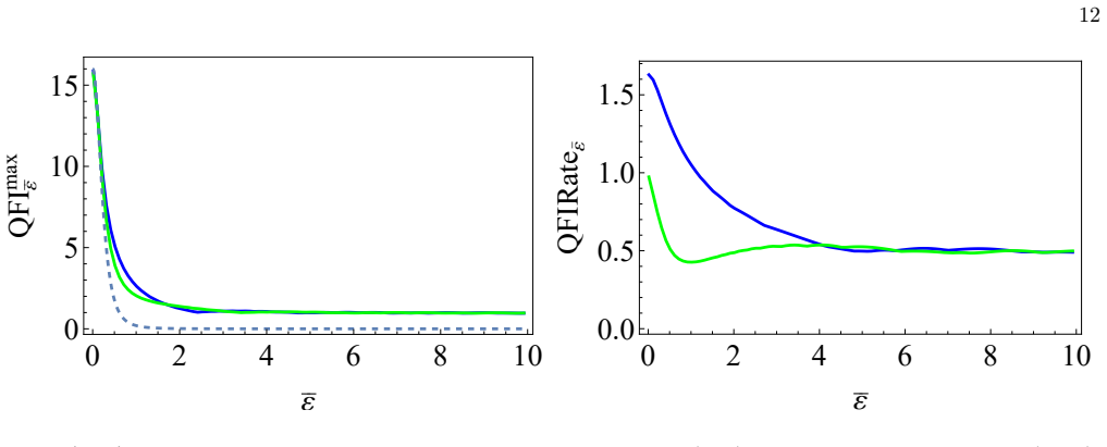
The optimal QFI Asthefirstquantityofinterest, wediscussthemaximal QFI reached by the atomic state (at some optimal time s) QFImax ¯ε = sup s QFI[ρs|¯ε].(83) The QFI of the stateρs|¯εcan also be computed analyti- cally. It admits a particularly simple expression at¯ε= 0, where for the ground and excited initial states one finds (see App. H for an arbitrary...
-
[8]
The steady-state QFI Next, let us consider the steady stateρ∗ ¯εof the dynam- ics. Solving0 =−i ¯ε[σy, ρ∗ ¯ε]+L σ−[ρ∗ ¯ε]we find the atomic steady-state read ρ∗ ¯ε= 1 2 1+ 1 1 + 8¯ε2 σz + 4¯ε 1 + 8¯ε2 σx ,(86) and gives QFI[ρ∗ ¯ε] = 4 (1 + 8 ¯ε2) 2 .(87) The QFI of the steady state is equal to16at¯ε= 0and vanishes in the limit of large¯ε, where the steady...
-
[9]
The optimal QFI rate In the limit where the total interaction time is very long, the best possible strategy (from the Fisher informa- tion perspective) is to repeat the measurement procedure for which the QFI rate is maximized QFIRate¯ε:= sup s QFI[ρs|¯ε] s ,(88) see e.g. Refs. [43, 46, 47]. In Fig. 5 (right panel), the maximal QFI rate as a function of¯ε...
-
[10]
The impact ofκ Finally, let us interpret these results in terms of the physical timet= s κ and the physical amplitudeε= √κ¯ε. For a stateρ ε we denote the QFI with respect to the εas gQFI[ρε]. To relate it to the quantities computed above, note that the parameter rescaling givesgQFI[ρε] = 1√κQFI[ρ¯ε=ε/√κ]. For a single interaction, the maximal reachable Q...
-
[11]
C. M. Caves,Quantum-mechanical noise in an interfer- ometer,Physical Review D23, 1693 (1981)
work page 1981
-
[12]
D. J. Wineland, J. J. Bollinger, W. M. Itano, F. Moore, and D. J. Heinzen,Spin squeezing and reduced quan- tum noise in spectroscopy,Physical Review A46, R6797 (1992)
work page 1992
-
[13]
M. J. Holland and K. Burnett,Interferometric detection of optical phase shifts at the Heisenberg limit,Physical Review Letters71, 1355 (1993)
work page 1993
-
[14]
V. Giovannetti, S. Lloyd, and L. Maccone,Quantum- enhanced measurements: beating the standard quantum limit,Science306, 1330 (2004)
work page 2004
-
[15]
M. G. Paris,Quantum estimation for quantum technol- ogy,International Journal of Quantum Information7, 125 (2009)
work page 2009
-
[16]
J. Aasi, J. Abadie, B. Abbott, R. Abbott, T. Abbott, M. Abernathy, C. Adams, T. Adams, P. Addesso, R. Ad- hikari,et al.,Enhanced sensitivity of the LIGO gravi- tational wave detector by using squeezed states of light, Nature Photonics7, 613 (2013)
work page 2013
-
[17]
R. Demkowicz-Dobrzański, K. Banaszek, and R. Schn- abel,Fundamental quantum interferometry bound for the squeezed-light-enhanced gravitational wave detector GEO 600,Physical Review A88, 041802 (2013)
work page 2013
-
[18]
F. Wolfgramm, A. Cere, F. A. Beduini, A. Predojević, M. Koschorreck, and M. W. Mitchell,Squeezed-light op- tical magnetometry,PhysicalReviewLetters105,053601 (2010)
work page 2010
-
[19]
B.-B. Li, J. Bílek, U. B. Hoff, L. S. Madsen, S. Forstner, V. Prakash, C. Schäfermeier, T. Gehring, W. P. Bowen, and U. L. Andersen,Quantum enhanced optomechanical magnetometry,Optica5, 850 (2018)
work page 2018
- [20]
-
[21]
M. Kacprowicz, R. Demkowicz-Dobrzański, W. Wasilewski, K. Banaszek, and I. Walmsley, Experimental quantum-enhanced estimation of a lossy phase shift,Nature Photonics4, 357 (2010)
work page 2010
-
[22]
I. I. Rabi,Space quantization in a gyrating magnetic field, Physical Review51, 652 (1937)
work page 1937
-
[23]
S.L.BraunsteinandC.M.Caves,Statistical distance and the geometry of quantum states,Physical Review Letters 72, 3439 (1994)
work page 1994
-
[24]
E. T. Jaynes and F. W. Cummings,Comparison of quan- tum and semiclassical radiation theories with applica- tion to the beam maser,Proceedings of the IEEE51, 89 (1963)
work page 1963
-
[25]
A. D. Greentree, J. Koch, and J. Larson,Fifty years of Jaynes–Cummings physics,Journal of Physics B: Atomic, Molecular and Optical Physics46, 220201 (2013)
work page 2013
-
[26]
F. Ciccarello, S. Lorenzo, V. Giovannetti, and G. M. Palma,Quantum collision models: Open system dynam- ics from repeated interactions,Physics Reports954, 1 (2022)
work page 2022
-
[27]
R. L. Berger and G. Casella,Statistical inference (Duxbury, 2001)
work page 2001
-
[28]
C. R. Rao, inBreakthroughs in Statistics: Foundations and basic theory(Springer, 1992) pp. 235–247. 15
work page 1992
-
[29]
Cramér,Mathematical methods of statistics, Vol
H. Cramér,Mathematical methods of statistics, Vol. 26 (Princeton university press, 1999)
work page 1999
-
[30]
Y. Ye and X.-M. Lu,Quantum Cramér-Rao bound for quantum statistical models with parameter-dependent rank,Physical Review A106, 022429 (2022)
work page 2022
- [31]
-
[32]
D. Šafránek,Discontinuities of the quantum Fisher in- formation and the Bures metric,Physical Review A95, 052320 (2017)
work page 2017
-
[33]
R. R. Rodríguez, M. Perarnau-Llobet, and P. Sekatski, TBD,In preparation (2025)
work page 2025
-
[34]
C. C. Gerry and P. L. Knight,Introductory quantum op- tics(Cambridge university press, 2023)
work page 2023
-
[35]
P. Sekatski, B. Sanguinetti, E. Pomarico, N. Gisin, and C. Simon,Cloning entangled photons to scales one can see,Physical Review A82, 053814 (2010)
work page 2010
-
[36]
J. Gea-Banacloche,Collapse and revival of the state vec- tor in the Jaynes-Cummings model: An example of state preparation by a quantum apparatus,Physical Review Letters65, 3385 (1990)
work page 1990
-
[37]
G. Zhang, G.-R. Li, and Z. Song,Quantum-state transfer between atom and macroscopically distinguishable cavity field in Jaynes–Cummings model,International Journal of Quantum Information13, 1550001 (2015)
work page 2015
-
[38]
J. H. Eberly, N. Narozhny, and J. Sanchez-Mondragon, Periodic spontaneous collapse and revival in a simple quantum model,PhysicalReviewLetters44,1323(1980)
work page 1980
- [39]
-
[40]
S. Phoenix and P. Knight,Fluctuations and entropy in models of quantum optical resonance,Annals of Physics 186, 381 (1988)
work page 1988
-
[41]
M. Fleischhauer and W. P. Schleich,Revivals made sim- ple: Poisson summation formula as a key to the revivals in the Jaynes-Cummings model,Physical Review A47, 4258 (1993)
work page 1993
-
[42]
Cummings,Stimulated emission of radiation in a sin- gle mode,Physical Review140, A1051 (1965)
F. Cummings,Stimulated emission of radiation in a sin- gle mode,Physical Review140, A1051 (1965)
work page 1965
-
[43]
J. Gea-Banacloche,Atom- and field-state evolution in the Jaynes-Cummings model for large initial fields,Phys. Rev. A44, 5913 (1991)
work page 1991
- [44]
-
[45]
B. Shore and P. Knight,The Jaynes–Cummings revival, Physics and Probability , 15 (1993)
work page 1993
-
[46]
H. Azuma,Application of Abel–Plana formula for collapse and revival of Rabi oscillations in Jaynes– Cummings model,International Journal of Modern Physics C21, 1021 (2010)
work page 2010
-
[47]
P. Berman and C. R. Ooi,Collapse and revivals in the Jaynes-Cummings model: an analysis based on the Mollow transformation,Physical Review A89, 033845 (2014)
work page 2014
-
[48]
Pavlik,Inside the Jaynes–Cummings sum,Physica Scripta99, 015113 (2023)
S. Pavlik,Inside the Jaynes–Cummings sum,Physica Scripta99, 015113 (2023)
work page 2023
-
[49]
P. Sekatski and M. Perarnau-Llobet,Optimal nonequi- librium thermometry in Markovian environments,Quan- tum6, 869 (2022)
work page 2022
-
[50]
K. A. Fischer, R. Trivedi, V. Ramasesh, I. Siddiqi, and J. Vučković,Scattering into one-dimensional waveguides from a coherently-driven quantum-optical system,Quan- tum2, 69 (2018)
work page 2018
-
[51]
A. Dąbrowska, D. Chruściński, S. Chakraborty, and G. Sarbicki,Eternally non-Markovian dynamics of a qubit interacting with a single-photon wavepacket,New Journal of Physics23, 123019 (2021)
work page 2021
-
[52]
zur quantentheorie der strahlung,inQuan- tentheorie(De Gruyter, Berlin, Boston, 1969) pp
A.Einstein,7. zur quantentheorie der strahlung,inQuan- tentheorie(De Gruyter, Berlin, Boston, 1969) pp. 209– 228
work page 1969
-
[53]
P. Sekatski, M. Skotiniotis, J. Kołodyński, and W. Dür, Quantum metrology with full and fast quantum control, Quantum1, 27 (2017)
work page 2017
-
[54]
R. Demkowicz-Dobrzański, J. Czajkowski, and P. Sekatski,Adaptive quantum metrology under general Markovian noise,Physical Review X7, 041009 (2017)
work page 2017
-
[55]
S. Zhou, M. Zhang, J. Preskill, and L. Jiang,Achieving the Heisenberg limit in quantum metrology using quantum error correction,Nature Communications9, 78 (2018)
work page 2018
-
[56]
L. A. Correa, M. Mehboudi, G. Adesso, and A. San- pera,Individual quantum probes for optimal thermome- try,Physical Review Letters114, 220405 (2015)
work page 2015
-
[57]
M. Mehboudi, A. Sanpera, and L. A. Correa,Thermom- etry in the quantum regime: recent theoretical progress, Journal of Physics A: Mathematical and Theoretical52, 303001 (2019)
work page 2019
-
[58]
R. Courant and D. Hilbert,Methods of Mathematical Physics, Vol. 1 (Wiley, New York, 1989)
work page 1989
-
[59]
N. L. Johnson, A. W. Kemp, and S. Kotz,Univariate discrete distributions(John Wiley & Sons, 2005)
work page 2005
-
[60]
√ ˆn α cos τ √ ˆn+ 1 sin τ √ ˆn # z(e) α = 1−2E h cos2(τ √ ˆn+ 1) i (C18) ˙x(e) α =−2E
F. Schäfer, P. Sekatski, M. Koppenhöfer, C. Bruder, and M. Kloc,Control of stochastic quantum dynamics by dif- ferentiable programming,Machine Learning: Science and Technology2, 035004 (2021). 16 Appendix A: QFI of a two-dimensional system For a general two dimensional stateρθ = aθ bθ −ic θ bθ + icθ 1−a θ , and its derivative˙ρθ ≡ ∂ρθ ∂θ = ˙aθ ˙bθ −i ˙cθ ...
work page 2021
-
[61]
The linear phase regime When the interaction timeτis relatively slow, the phases are well approximated by linear functions on the support of the Poissonian distributions. More precises expanding inˆδ= ˆn−α2 α =O(1)one finds S0(n), S1(n), S2(n) = 2ατ+τ n−α 2 α +τ O(α −1)(D5) S3(n) =− τ 2α + τ 4α2 n−α 2 α +τ O(α −3).(D6) Using the moment generating function...
-
[62]
(D4), we follow the approach presented in [31]
The rapid phases regime In the limit where the linear phase approximation fails, to compute such sums in the right-hand side of Eq. (D4), we follow the approach presented in [31]. For simplicity we now focus on the phases fork= 0,1,2and come back to the casek= 3at the end of the section. First, we use the Poissonian summation [48] to express the discrete ...
-
[63]
The full reduced dynamics of the atom Summarizing the above calculations, we find that in the limit of largeαwith τ/α3 →0and up toO(α −1)the expected values in Eq. (D4) are given by ∞X n=0 P(n|α)Γ ij(n)eiSk(n) ≈ P∞ ν=0 I0,ν k= 0,1P∞ ν=0 I0,ν(−1)ν k= 2P∞ ν=0 I3,ν k= 3 ,(D24) with all the terms given in Eqs. (D17, D8, D7). This allows us to express ...
-
[64]
Quantum Fisher information at short timesτ=O(1) Forτ≪αusing Eq
The atomic state and its QFI To discuss the final state for an atom prepared in the ground or excited state and its QFI, we again separately consider the three different time regimes a. Quantum Fisher information at short timesτ=O(1) Forτ≪αusing Eq. (D31) one immediate obtainsx (g/e) τ|α =±e −τ 2/2 sin(2ατ),z (g/e) τ|α =±e −τ 2/2 cos(2ατ)(where the sign±i...
-
[65]
1−τ 2(α2 + 1)−τ α τ α −τ α−τ α τ 2(α2 + 1)−τ 2α2 τ α τ α−τ 2α2 τ 2α2 = 1 1−αdt αdt 1 1−αdt αdt −αdt−αdt0 0 αdt αdt0 0 +O(dt 2)(F1) so the atomic dynamics is unitary d dt ρt|ε =−iα[σ y, ρt|ε].(F2) Appendix G: The continuous quantum field limit In this section, we compute the limit where the interaction parameter for a single discrete mode i...
-
[66]
1−τ 2(⟨ˆn⟩+ 1)−τ a† τ⟨a⟩ −τ⟨a⟩ −τ⟨a⟩τ 2(⟨ˆn⟩+ 1)−τ 2 a†2 τ a† τ a† −τ 2 a2 τ 2 ⟨ˆn⟩ ,(G5) where the expected values⟨A⟩= trA|F⟩ ⟨F|are taken on the initial state of the incident radiation mode. Taking the field mode in the coherent state|α⟩= ε √ dt E , we further obtainG= ˜G+O((τ α) 3)with ˜G= 1−τ 2α2 1−τ 2(α2 + 1 2)−τ α τ α 1−τ 2(α2 + 1
-
[67]
1−τ 2(α2 + 1)−τ α τ α −τ α−τ α τ 2(α2 + 1)−τ 2α2 τ α τ α−τ 2α2 τ 2α2 = 1 1− κdt 2 −√κεdt √κεdt 1− κdt 2 1−κdt− √κεdt √κεdt −√κεdt− √κεdt κdt0√κεdt √κεdt0 0 ,(G6) where we only kept the leading orders indtin the last expression. It is then straightforward to verify that the resulting channel is of the form Edt|ε[•] = 3X i,j=0 Gji Li •L † ...
discussion (0)
Sign in with ORCID, Apple, or X to comment. Anyone can read and Pith papers without signing in.