REVIEW 4 major objections 6 minor 10 references
A Numerical Rosenblatt Method for Forced Variable Independence
T0 review · 4 major / 6 minor · reviewed 2026-08-15 · deepseek-v4-flash
Pith's one-line read A numerical Rosenblatt transform can force a classifier to be statistically independent of a chosen observable, and the transformed classifier keeps its separation power.
desk verdict A post-processing Rosenblatt transform that beats DisCo at preserving AUC in their LHC Olympics test; mathematically sound, empirically promising, but the same-density assumption is untested. read the letter →
The pith
A machine-rendered reading of the paper's core claim, the machinery that carries it, and where it could break.
The reading
What carries the argument
The load-bearing object is the conditional cumulative distribution transform $\gamma(x,y)$ of Eq. (4): the $y$-normalized primitive of the joint density $\rho$ along the $y$-axis, $\gamma(x,y)=\int_{-\infty}^{y} \rho(x,y')\,dy'/\int_{-\infty}^{\infty} \rho(x,y'')\,dy''$. It is the same object as the classical Rosenblatt transform, re-derived independently here. Its role is to map, for every fixed $x$-slice, the conditional distribution of $y$ onto a uniform distribution; the change-of-variable calculation in Appendix A then makes the joint density factor as $\rho_X(x)\cdot 1_{(0,1)}(\gamma)$, which is exactly independence. The paper's numerical contribution is to estimate this transform from a finite background sample by two routes: IRGI, which builds an irregular equal-count grid and uses normalized cumulative column sums, and KDE, which replaces the density by Gaussian kernels with the ratio of smoothing widths controlled by a free parameter $\sigma_r$.
What would settle it
Train the transform on one background sample and apply it to a second sample generated from a different but plausible background density, for example the same process with a shifted calorimeter energy scale; if the measured DCC between $x$ and $\gamma$ in the second sample stays at the original $(x,y)$ level rather than dropping toward $10^{-4}$, the practical quasi-independence claim fails.
Extended reading notes
Core claim
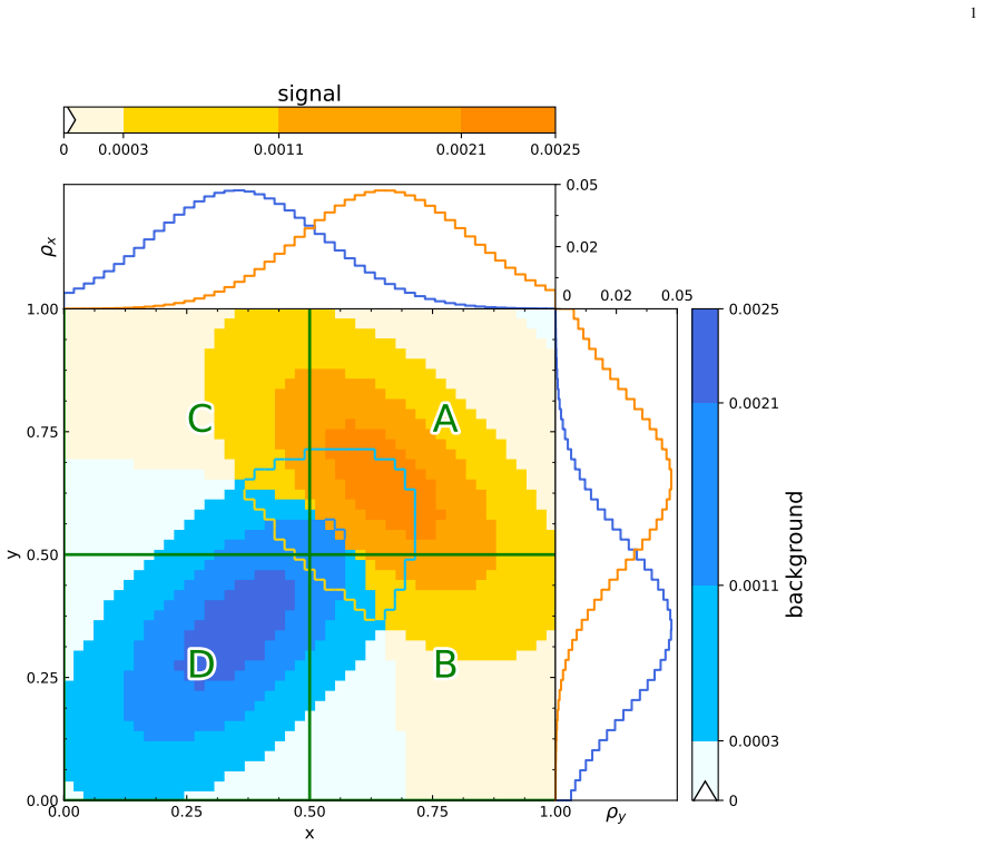
The paper's central claim is that the numerical conditional-CDF transform of Eq. (4), $\gamma(x,y)$, renders its output independent of $x$: for any continuous background density $\rho$, the transformed joint density satisfies $\rho(x,\gamma)=\rho_X(x)\cdot 1_{(0,1)}(\gamma)$. Because of this, applying the transform to the output of an arbitrary classifier makes the classifier quasi-independent of the observable while preserving the classifier's ordering of events; the ROC curve changes minimally. On the LHC Olympics dijet example, the IRGI version reaches DCC $0.00025$ with AUC $0.912$ and the KDE version DCC $0.00018$ with AUC $0.911$, compared with baseline $0.01658$/$0.911$ and a DisCo classifier at DCC $0.00011$ whose AUC drops to $0.828$.
Load-bearing premise
The defining background sample used to estimate the conditional CDF must be representative of the background events in the actual analysis; if simulation or sideband data disagrees with real background, the transform is miscalibrated and $\gamma$ will not be independent in practice.
Editorial extensions
If this is right
- Any trained classifier can be post-processed into a background-quasi-independent score, so the independence requirement no longer has to be baked into the loss function during training.
- In the paper's LHC Olympics example, the transformed classifier keeps AUC $0.912$ (baseline $0.911$) while pushing DCC down by two orders of magnitude, so ABCD-style background estimation can be applied without a resolution-power penalty.
- The method works on the defining background sample alone; signal events are not used to build the transform, which makes it applicable to control-region or simulation-based background definitions.
- Both IRGI and KDE reduce DCC consistently across five independent subsamples in the toy test, and the ABCD relative error in signal estimation for the IRGI-transformed classifier is roughly three times smaller than for the baseline in the paper's setup.
Reading between the lines
- Because the transform is built from background only, it should transfer to anomaly-detection settings where signal is unknown: the same conditional CDF can define a background-independent coordinate for weakly supervised searches, and a classifier trained or cut on it would inherit the independence property by construction.
- The construction treats the defining background sample as ground truth; a natural robustness test would be to build $\gamma$ on one background simulation and apply it to a second simulation of the same process with different detector response or generator settings, then measure whether the DCC stays near zero.
- The independence proof requires the true density and exact integration; with finite samples the numerical estimators can only approximate $\gamma$, so the practical limit on DCC is set by sample size, smoothing width, and grid depth rather than by the method itself.
- A direct comparison with the ABCDisCo variant at matched DCC, using the authors' own ABCD relative-error metric, would clarify how much of the gain comes from avoiding retraining instability and how much from the transform's exact factorization.
Signed reviews
Editorial analysis
A structured set of objections, weighed in public.
Referee Report
Summary. The paper proposes a numerical method for transforming a random variable y into a new variable γ defined as the conditional cumulative distribution function of y given an observable x under a background probability density. The transformation (Eq. 4) is a Rosenblatt transform; the authors prove in Appendix A that γ is independent of x and marginally uniform on [0,1]. Two numerical estimators are presented: IRGI, based on irregular adaptive binning with linear interpolation, and KDE, based on Gaussian kernel smoothing. The method is intended as a plug-in decorrelation layer for classifiers in particle physics, replacing training-time constraints such as DisCo. The authors demonstrate the method on a Gaussian toy example, a cat/dog image classification task with a color observable, and an LHC Olympics dijet dataset, reporting lower distance correlation at comparable or higher AUC than DisCo in the LHC example.
Significance. The mathematical foundation is sound: the independence result follows from the classical Rosenblatt transform, and the proof in Appendix A is correct under the stated regularity conditions. The numerical implementations are clearly described and the LHC Olympics example is a relevant stress test. If the reported performance holds out-of-sample, the method offers a simple, model-agnostic alternative to DisCo with a rigorous independence guarantee and no adversarial optimization. However, the empirical validation is currently weakened by in-sample parameter selection (the DCC minima are obtained on the same data used to select d and σ_r) and by the absence of statistical uncertainties on DCC and AUC. In addition, the paper does not test robustness to mismodeling of the defining background sample, which is the key assumption for practical use. These issues are fixable and do not invalidate the core idea.
major comments (4)
- [III.C, Figs. 17-18] The DCC values reported for the IRGI and KDE classifiers (DCC 0.00025 and 0.00018, respectively) are the result of scanning the free parameters d and σ_r on the same 20k-event validation sample that is used to compute these DCC values. The minimum over a parameter grid is an in-sample optimum and is expected to be smaller than the performance on unseen data. The paper does not report DCC on the held-out testing sample (100k background, 10k signal) used for the ABCD demonstration. To support the central claim, the authors should either report DCC on the testing sample or use a nested cross-validation scheme where parameter selection is performed on a training slice and DCC is evaluated on an independent slice.
- [III.A, Table III-A, Figs. 8-9] In the Gaussian blob example, for each of the five subsamples the DCC minima for IRGI and KDE are obtained by scanning d or σ_r on that same subsample, so the reported minima are biased estimates of the method's DCC. Additionally, no statistical uncertainties (bootstrap or repeated draws) are reported for DCC or AUC, so it is unclear whether the differences between IRGI, KDE, and the baseline are statistically significant. The authors should provide confidence intervals or per-repetition variations, and ideally a separate validation set for parameter selection.
- [II (defining background sample) and III.C] The independence guarantee is conditional on the defining background sample being drawn from the same underlying probability density as the evaluation sample. The paper states this assumption but does not assess its robustness. In the LHC Olympics example the defining sample and the evaluation sample are both from the same Monte Carlo generator, so the demonstration does not cover the realistic scenario in which the simulation used to construct the transform does not perfectly describe the data (e.g., miscalibrated mass spectrum or mismodeled track features). A robustness study with a perturbed defining sample is necessary to support the practical claim that the method renders a classifier quasi-independent in an actual analysis.
- [II.A (IRGI algorithm), Fig. 4] The IRGI algorithm constructs the transform on a finite rectangular defining domain, with interpolation vertices placed on the domain boundary. The paper does not specify how the transform is evaluated for points outside this domain, nor how it behaves when the evaluation sample extends beyond the support of the defining sample. In the LHC Olympics example, the observable x extends beyond the region shown in the defining sample; an explicit extrapolation rule is needed to define γ for those events.
minor comments (6)
- [II.A] The acronym 'IRregular' should be 'Irregular' or the capitalization should be explained, as 'IRregular Grid Interpolation' is unusual.
- [V] In the acknowledgements, 'independetly' should be 'independently'.
- [III.C] The phrase 'bump-hunt is inpired' should be 'inspired'.
- [Various] The abbreviation 'TMV A' appears throughout the text; it should be written consistently as 'TMVA'.
- [II.B, Eq. (8)] The phrase 'unique pairs (xi,xj)' is ambiguous; it should specify all pairs with i<j.
- [Figures 5, 30, 31] Several subfigures lack complete captions; for example, Fig. 5(b) has no description after the label.
Circularity Check
The Rosenblatt independence proof is self-contained, but the headline DCC improvements are minima selected on the same validation data, so the empirical 'predictions' are partly fitted.
-
fitted input called prediction
[Section III.A, Figs. (8)-(9) and Tab. (III-A)]
"For each subsample, (x,y)-DCC is computed and compared with (x,γ_d)-DCC and (x,γ_σr)-DCC for varying free parameters. ... DCC minima found per sample for both numerical techniques, are summarized in Tab. (III-A). We observe that in each subsample, for IRGI parameter d found to minimize the DCC of x and the modified classifier; KDE parameter σ_r can be found to surpass, or be equal to, the IRGI."
The tabulated DCC(x,γ_d) and DCC(x,γ_σr) are the minima over the scanned d or σ_r computed on the same five testing subsamples. Thus the reported 'achieved' DCC is the objective being minimized, not an independent evaluation at a fixed parameter; it is small by construction of the scan. This does not impugn the Rosenblatt independence theorem, but it means the numerical demonstration's headline DCC values are fitted, not predicted.
-
fitted input called prediction
[Section III.C, Figs. (17)-(18) and surrounding text]
"Additionally, 20k background and signal events form validation samples for free parameter optimization (minimizing DCC, maximizing AUC). ... DCC-optimal IRGI and KDE parameters are found as d=6 and σ_r=0.024 ... BL classf., DCC: 0.01658, AUC: 0.911; mod. classf. IRGI_6, DCC: 0.00025, AUC: 0.912; mod. classf. KDE_0.024, DCC: 0.00018, AUC: 0.911."
The same 20k validation sample is used both to choose the free parameters by minimizing DCC and to report the DCC/AUC values in Fig. 18. The DCC 0.00025 is therefore the minimum of the scanned grid on that sample, i.e. the selection criterion itself, not a fixed-parameter prediction on an independent test set. The comparison to DisCo is likewise made after selecting the DisCo point on the same plane, so the claimed superiority is in part an artifact of selection on the evaluation sample.
full rationale
The central mathematical derivation is not circular. Appendix A proves, by a direct Jacobian computation from the definition of the conditional-CDF transform in Eq. (4), that ρ(x,γ) factors as ρ_X(x) times the uniform density; this is the standard Rosenblatt argument and does not assume the conclusion. The paper's citation of Rosenblatt is external and non-self-referential, and no uniqueness theorem is imported from the authors' own prior work. The two flagged steps concern the numerical evaluation: in both the blob example and the LHC Olympics example, the free parameters d and σ_r are explicitly chosen to minimize DCC on the same validation subsamples that then supply the reported DCC minima. Those reported numbers are therefore optimized values on the evaluation set, not out-of-sample predictions at fixed parameter values. This is a real selection-bias circularity in the empirical demonstration, but it does not affect the correctness of the underlying transform. The untested assumption that the defining background sample matches the true background density is a correctness/robustness risk, not a circularity. Overall, the core independence claim has independent mathematical content, while the headline numerical DCC improvements are partly fitted on the validation data, giving a moderate score of 4.
Assumptions & free parameters
free parameters (3)
- IRGI recursive bisection depth d =
d=7 (Gaussian blobs), d=4 (cats/dogs), d=6 (LHC Olympics)
- KDE relative kernel width sigma_r =
sigma_r around 0.05-0.1 (Gaussian and cats/dogs), 0.024 (LHC Olympics)
- ABCD quadrant boundary (x0,y0) =
optimized per classifier over x0 in [2.0,3.7] and y0 in [0.1,0.85]
assumptions (3)
- domain assumption Underlying probability densities for background and signal exist, and the defining background sample is drawn from the same density as the test background.
- domain assumption The background density rho(x,y) is absolutely continuous and the marginal rho_X(x) is nonzero on the defining x-domain.
- domain assumption The classifier output y is treated as a continuous random variable so the conditional CDF is strictly monotone and invertible.
Cite this review
Pith. "Pith review of A Numerical Rosenblatt Method for Forced Variable Independence." pith.science (2026). https://pith.science/paper/SOHTMPRP
@misc{pith2026250925521,
  author       = {Pith},
  title        = {Pith review of: A Numerical Rosenblatt Method for Forced Variable Independence},
  year         = {2026},
  howpublished = {\url{https://pith.science/paper/SOHTMPRP}},
  note         = {Machine review of arXiv:2509.25521}
}
read the original abstract
A novel numerical technique is presented to transform one random variable within a system toward statistical quasi-independence from any other random variable in the system. The method's applicability is demonstrated through a particle physics example where a classifier is rendered quasi-independent from an observable quantity.
Figures


Figures from the paper (28 more)


Reference graph
Works this paper leans on
-
[1]
2025.DOI: 10.48550/ARXIV .2506.08826.URL: https://arxiv.org/abs/2506.08826
CMS Collaboration.Machine learning method for enforcing variable independence in background estimation with LHC data: ABCDisCoTEC. 2025.DOI: 10.48550/ARXIV .2506.08826.URL: https://arxiv.org/abs/2506.08826
-
[2]
Measuring and testing dependence by correlation of distances
Gábor J. Székely, Maria L. Rizzo, and Nail K. Bakirov. “Measuring and testing dependence by correlation of distances”. In:The Annals of Statistics35.6 (Dec. 2007).ISSN: 0090-5364.DOI: 10.1214/009053607000000505.URL: http://dx.doi. org/10.1214/009053607000000505
-
[3]
ROC Solid: Receiver Operator Characteristic (ROC) Curves as a Foundation for Better Diagnostic Tests
Mark R. J. Junge and Joseph R. Dettori. “ROC Solid: Receiver Operator Characteristic (ROC) Curves as a Foundation for Better Diagnostic Tests”. In:Global Spine Journal8.4 (May 2018), pp. 424–429.ISSN: 2192-5690.DOI: 10.1177/ 2192568218778294.URL: http://dx.doi.org/10.1177/2192568218778294
-
[4]
Remarks on a Multivariate Transformation
Murray Rosenblatt. “Remarks on a Multivariate Transformation”. In:The Annals of Mathematical Statistics23.3 (Sept. 1952), pp. 470–472.ISSN: 0003-4851.DOI: 10.1214/aoms/1177729394.URL: http://dx.doi.org/10.1214/aoms/1177729394
arXiv 1952
-
[5]
Albertsson.Users Guide - TMVA 4 - ROOT - CERN
K. Albertsson.Users Guide - TMVA 4 - ROOT - CERN. 2007.URL: https : / / root . cern . ch / download / doc / tmva / TMV AUsersGuide.pdf
work page 2007
-
[6]
2025.URL: https://www.cs.toronto.edu/~kriz/cifar.html
Alex Krizhevsky.CIFAR10 dataset. 2025.URL: https://www.cs.toronto.edu/~kriz/cifar.html
work page 2025
-
[7]
Software available from tensorflow.org
Martín Abadi et al.TensorFlow: Large-Scale Machine Learning on Heterogeneous Systems. Software available from tensorflow.org. 2015.URL: https://www.tensorflow.org/
work page 2015
-
[8]
2019.URL: https://zenodo.org/records/2629073
Gregor Kasieczka, Ben Nachman, and David Shih.R&D Dataset for LHC Olympics 2020 Anomaly Detection Challenge. 2019.URL: https://zenodo.org/records/2629073
Show all 10 references
-
[9]
Anomaly detection with density estimation
Benjamin Nachman and David Shih. “Anomaly detection with density estimation”. In:Physical Review D101.7 (Apr. 2020).ISSN: 2470-0029.DOI: 10.1103/physrevd.101.075042.URL: http://dx.doi.org/10.1103/PhysRevD.101.075042. APPENDIXA MATHEMATICALTREATMENT OF THETECHNIQUE Consider the...
2020 doi
-
[10]
(19), the marginal distributionρ X(x), must be non-zero on the definingx-interval
The denominator in Eq. (19), the marginal distributionρ X(x), must be non-zero on the definingx-interval. To demonstrateγ’sx-independence, substitute into Eq. (16): JΓ−1(x,γ) = ∂x ∂x ∂x ∂γ ∂y(x,γ) ∂x ∂y(x,γ) ∂γ ! JΓ−1(x,γ) = 1 0 ∂y(x,γ) ∂x ∂γ(x,y) ∂y (x,γ) −1 ! |detJΓ−1(x,γ)|=...
Reviewed August 15, 2026 · model on record in the stance chip above.
Discussion (0). Continue with ORCID to comment.