Introduction to Model-Based Derivative-Free Optimization

Lindon Roberts

REVIEW 1 major objections 5 minor 1 cited by

Introduction to Model-Based Derivative-Free Optimization

T0 review · 1 major / 5 minor · reviewed 2026-08-04 · deepseek-v4-flash

Challenge this review Re-run · record.json Download PDF Read on arXiv ↗

Pith's one-line read Without derivatives, interpolation methods match trust-region rates, a new survey proves, with explicit dimension factors.

desk verdict A careful, honest, current introduction to interpolation-based DFO; the proofs are sound, and the limitations are stated plainly. read the letter →

arxiv 2510.04473 v2 pith:YFX6AS2V submitted 2025-10-06 math.OC

Lindon Roberts This is my paper · ORCID

classification math.OC MSC 90C5665K05

keywords derivative-freeoptimizationinterpolation-basedtrust-regionmethodsworst-casecomplexityfullylinearmodelsquadraticpoisedinterpolationsetsnoisy

verification ladder T0 review T1 audit T2 compute T3 formal

The pith

A machine-rendered reading of the paper's core claim, the machinery that carries it, and where it could break.

The reading

The paper is a systematic introduction to interpolation-based optimization (IBO), the branch of derivative-free optimization that replaces Taylor models with models built from function values. Its central thesis is that the standard trust-region machinery survives intact when derivatives are removed: if each local model is fully linear or fully quadratic with uniform constants, then simple IBO algorithms converge to first-order points in O(n ε^-2) iterations and to second-order points in O(n^3 ε^-3) iterations, matching derivative-based complexity up to explicit dimension factors. To make this concrete, the paper develops interpolation theory—linear, quadratic, minimum-Frobenius-norm, and regression models—and shows how poised interpolation sets certify the required model accuracy. It then extends the framework to convex constraints via feasible interpolation and to deterministic and stochastic noise, deriving an accuracy floor for bounded deterministic noise and high-probability complexity for stochastic noise. A sympathetic reader gains a self-contained map of what is guaranteed for model-based derivative-free optimization and which assumptions carry the rates.

What carries the argument

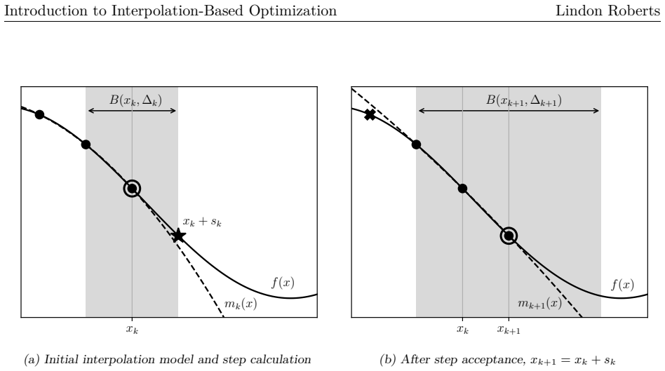
The load-bearing pair is the definitions of fully linear and fully quadratic models—error bounds that scale as Δ² and Δ³ over the trust region—and Lagrange polynomials with Λ-poisedness, which certify those bounds for interpolation sets. The trust-region algorithm itself is the derivative-based method with an added criticality check that reconnects the model gradient, which can be small even when the true gradient is not, to the true optimality measure. The interpolation constructions, including coordinate perturbations, minimum-Frobenius-norm underdetermined quadratics, and self-correcting geometry updates, are what make the fully linear and fully quadratic assumptions achievable, and the c

What would settle it

Run the simple IBO algorithm on a smooth two-dimensional function while deliberately reusing interpolation points so the interpolation set becomes increasingly ill-poised and the fully-linear constant grows with each accepted step; if the iteration count to reach ∥∇f∥ < ε grows slower than the predicted O(ε^-2), the uniform-constant assumption is not necessary, and if it degrades, the stated rates are tight to that assumption.

Watch

Extended reading notes

Core claim

The central claim is that interpolation-based optimization inherits the convergence theory of trust-region methods provided the interpolation model is fully linear or fully quadratic in the trust region with constants independent of the iteration. Under that condition, the simple IBO algorithm has O(n ε^-2) first-order iteration complexity and the second-order variant has O(n^3 ε^-3) complexity, with objective-evaluation counts O(n^2 ε^-2) and O(n^5 ε^-3). The paper's contribution as an expository treatment is to prove these bounds from first principles: the fully linear and fully quadratic error bounds follow from interpolation theory, and the interpolation theory is controlled by the poise

Load-bearing premise

The rates rest on the assumption that at every iteration the interpolation model is fully linear or fully quadratic with constants independent of k; the self-correcting geometry algorithm proves only liminf convergence and not a worst-case bound, so the sharp rates are guaranteed only when models are rebuilt or re-certified at full cost each iteration.

Editorial extensions

If this is right

If the model accuracy assumptions hold at every iteration, users get the same ε-scaling in iteration count as gradient-based trust-region methods: O(ε^-2) for first-order and O(ε^-3) for second-order stationary points.
Dimension enters explicitly: linear interpolation costs O(n ε^-2) iterations and O(n^2 ε^-2) evaluations; fully quadratic interpolation costs O(n^3 ε^-3) iterations and O(n^5 ε^-3) evaluations.
Termination on a small trust-region radius is justified, giving practitioners a stopping rule that does not require access to ∇f.
In the constrained setting, feasible interpolation models with poisedness measured only inside the feasible region recover the unconstrained rates, fixing the pathological δ-dependence of naive feasible interpolation.
For bounded deterministic noise, the accuracy floor is ε_min = O(√ε_f): no algorithm of this type can be guaranteed below that, while stochastic noise with averaging recovers any accuracy with high probability.

Reading between the lines

Editorial extensions of the paper, not claims the author makes directly.

A consequence the paper leaves implicit: in the expensive-evaluation regime, the per-iteration evaluation counts, not the iteration counts, are the practical budget, and the self-correcting geometry algorithm trades some of that cost for a weaker guarantee—liminf convergence with no worst-case bound.
The uniform fully-linear-constants assumption is doing most of the work; a natural testable extension is to track how those constants grow when interpolation points are reused and to seek complexity bounds under controlled poisedness decay.
The deterministic-noise floor suggests a general principle for noisy black-box optimization: if noise is bounded but cannot be shrunk, one can only hope for a neighborhood of the solution, and the neighborhood radius scales with the square root of the noise level regardless of interpolation scheme.
The framework could be extended to a hybrid strategy that spends cheap single samples early and switches to large-N averaging only near criticality, potentially improving the O(ε^-6) stochastic evaluation complexity in practice.

Share X Bluesky LinkedIn Reddit HN

Editorial analysis

A structured set of objections, weighed in public.

Desk editor's note, referee report, and a circularity audit.

Desk Editor's Note

read the letter

This is a competent, honest, and useful introduction to interpolation-based optimization. It is not a research paper, but it does what it sets out to do: give a graduate student a rigorous, up-to-date pathway into the field. The novel content is modest — some reproofs of known results with tighter constants — but that is appropriate for the genre.

The mathematics holds up. I checked the main proof chains: the fully linear/quadratic error bounds, the complexity theorems, the geometry improvement argument, and the constrained feasibility argument. They are internally consistent and match the published sources. The exposition is actually better than the older book by Conn, Scheinberg, and Vicente in several places, especially in the treatment of worst-case complexity and in the separation of deterministic vs. stochastic noise. The paper is also honest about its own gaps: no worst-case complexity for the self-correcting Algorithm 6.2, the O(√ϵf) accuracy floor under deterministic noise, and the open Λ1-vs-Λ∞ question. That honesty is a strength, not a weakness.

Where are the soft spots? The main one is the gap between the algorithms that get the clean complexity rates (Assumptions 4.2/4.10, model rebuilt or certified every iteration) and the self-correcting algorithm that is more practical but lacks the worst-case bound. This is a known gap in the field, and the paper flags it explicitly in Section 6.3. It is not a hidden premise. Another minor issue: the typo in Lemma 4.12 (the direction of the inequality) could confuse a careful reader, though it doesn't affect the conclusion. The title mismatch between the arXiv metadata and the PDF is a metadata problem, not a content problem.

The citation pattern looks fine. The author cites his own prior work where appropriate, plus the standard references. For an introduction, the coverage is appropriately scoped — it does not pretend to be a comprehensive survey.

Who should read this? Students and researchers who want to get to the research frontier in model-based DFO. Experts will not find new results, but they will find a useful reference for teaching. I would send this to a serious referee: it deserves careful review, and it will likely become a standard reference. My recommendation is to accept after minor revisions (fix the typo, make the title consistent).

Referee Report

1 major / 5 minor

Summary. This paper is a self-contained introduction to interpolation-based optimization (IBO), the class of derivative-free trust-region methods that replace Taylor models with polynomial interpolation models built from zeroth-order evaluations. The first half develops the fully linear/fully quadratic model framework (Definitions 4.1 and 4.9) and proves first-order (Theorem 4.7) and second-order (Theorem 4.15) iteration-complexity bounds, O(κ_m²κ_H ε^{-2}) and O(κ_m(κ_m+κ_H)² ε^{-3}), under Assumptions 4.2/4.10. The second half supplies the approximation theory: linear and quadratic interpolation with explicit constants (Theorems 5.2 and 5.5; Corollaries 5.4 and 5.7), regression and minimum-Frobenius-norm underdetermined quadratic models (Theorems 5.9, 5.15; Corollary 5.16), and Lagrange-polynomial/Λ-poisedness tools for self-correcting geometry (Section 6). Extensions cover convex constraints via C-feasible fully linear models (Section 7.1), general constraints via an SQP outline (Section 7.2), deterministic noise with a modified ratio test and an O(√ϵ_f) accuracy floor (Theorem 8.7), and stochastic noise with sample averaging and an O(ϵ^{-6}) evaluation-complexity regime (Theorem 8.17).

Significance. If the results hold, this is a valuable pedagogical reference that sits between the Conn–Scheinberg–Vicente book and the Larson–Menickelly–Wild survey. Its main strengths are the explicit, non-asymptotic constants in every model-error bound (no fitted parameters), the complete proofs of the core complexity theorems, and the unusually candid limitation statements: Section 6.3 explicitly states that the self-correcting Algorithm 6.2 lacks a worst-case complexity bound; Theorem 8.7 explicitly carries the ϵ_min = O(√ϵ_f) noise floor; Section 7.2 notes that no general-constraint IBO method currently has both theory and practice. These disclosures allow a reader to see exactly where the theory stops. The scope restriction — that the sharp O(n ε^{-2}) / O(n³ ε^{-3}) rates require rebuilding or re-certifying interpolation points each iteration under Assumptions 4.2/4.10 — is the honest cost of the presented framework. The reader's weakest-assumption concern does not, on reading the paper, land as an error: the worst-case complexity theorems are explicitly conditional on Assumptions 4.2/4.10, Section 5 supplies concrete interpolation constructions satisfying them, and Section 6.3's caveat i

major comments (1)

[§5–6, Corollaries 5.4/5.7 vs §6.3] The abstract promises coverage of "worst-case complexity" for IBO, and the headline rates O(n ε^{-2}) and O(n³ ε^{-3}) require the model to be fully linear/quadratic at every iteration with constants independent of k (Corollaries 5.4 and 5.7). The paper's own self-correcting geometry machinery (Algorithm 6.2) is proved only to satisfy liminf convergence, with the text stating "We prove global convergence of the algorithm, but not worst-case complexity bounds" (§6.3). Thus the complexity claims do not cover the mechanism that would make interpolation-set management efficient in practice. This is not an internal inconsistency — the conditions are stated and the limitation is declared — but it is a scope restriction that should be stated in the introduction/abstract, not only in §6.3, so that a casual reader does not over-read the complexity coverage.

minor comments (5)

[Title/metadata] The arXiv listing gives the title as "Introduction to Model-Based Derivative-Free Optimization" but the first page and running header use "Introduction to Interpolation-Based Optimization"; please ensure the metadata, title page, and abstract are consistent.
[§4, Remark 4.3 and Algorithms 4.1/4.3] Remark 4.3 says that if ∥g_k∥ < µ_c ∆_k, "we may save our efforts by not solving the trust-region subproblem or evaluating f(x_k+s_k)", but Algorithm 4.1 (lines 3–4) always computes s_k and evaluates f(x_k+s_k) before the criticality check in lines 5–8. Algorithm 4.3 likewise always evaluates the trial point even when the iteration turns out to be model-improving. Either amend the pseudocode to perform the criticality check immediately after model construction, or revise the remark to note that the saving is not reflected in the pseudocode as written.
[§8.1–8.2, Theorem 8.7 and Lemma 8.16] Theorem 8.7 (deterministic noise) and Lemma 8.16 (drift condition for the stochastic analysis) are stated without proof, citing [19] and [12,27], respectively; Lemmas 6.11 and 7.15 likewise defer to [96]. For a paper that otherwise gives complete proofs of its core results, a short proof sketch for Theorem 8.7 and Lemma 8.16 would make the noisy sections more self-contained, or the text should label them as "beyond the scope of this introduction".
[§8.2, before Remark 8.18] The discussion says the algorithm "may require up to O(ϵ^{-4}) stochastic objective evaluations per iteration, or O(ϵ^{-6}/(α_m α_f − 1/2)) evaluations in total." The total count should include the number of interpolation points (p = O(n)) per model, giving O(n ϵ^{-6}) for fixed success probabilities; please clarify whether the displayed rate is iteration complexity and state the n-dependence.
[§2 and §6.2] Typos/wording: §2 "Lipchitz" should be "Lipschitz"; §6.2 Figure 6.1 caption's "The value of Λ∞ is still not unreasonably large here" is informal; in the Theorem 6.12 proof the step "min(|ℓ_i(y)|,ℓ_i(y)^2) > Λ*∞" relies on |ℓ_i(y)| > Λ*∞ > 1 and could be spelled out.

Circularity Check

0 steps flagged · score 2.0 of 10

No significant circularity: complexity theorems are conditional on independently verified interpolation-model assumptions; self-citations are bibliographic, not definitional.

full rationale

The paper is an expository survey, not a parametric fit. Its central first/second-order complexity results (Theorem 4.7, Corollaries 4.8/5.4; Theorem 4.15/Corollary 5.7) explicitly condition on Assumptions 4.2/4.10—fully linear/quadratic models with k-independent constants—and Section 5 then supplies self-contained constructions (linear interpolation to {xk, xk+Δke_i}; quadratic interpolation to the set (5.49)) with proved error bounds (Theorems 5.2, 5.5, Lemmas 5.3/5.6) that satisfy those assumptions. The error bounds are expressed in terms of matrix inverse norms and smoothness constants; they are not defined in terms of the target convergence rates. There are no fitted parameters and no empirically calibrated inputs. The few places where proofs are delegated to the author's prior work—e.g. Lemma 6.11 cites [96, Theorem 5.2], Theorem 7.10 cites [58, Theorem 3.14], Theorem 8.7 says it may be derived from [19, Theorem 4.11]—are citations to published theorems with stated assumptions that do not include the desired conclusion; they are therefore independent support rather than circularity. The manuscript also flags its own limitations honestly: Section 6.3 states 'We prove global convergence of the algorithm, but not worst-case complexity bounds' for Algorithm 6.2, and Theorem 8.7's proof is explicitly 'Omitted for brevity'. These passages reduce any impression that unsupported bounds are being claimed, and they do not create a reduction of a conclusion to an input. No step in the derivation chain equates a model assumption with a target result, and no uniqueness claim is imported from the authors' prior work to force a choice.

Assumptions & free parameters 2 free parameters · 8 assumptions · 2 invented entities

All axioms are standard for the derivative-free optimization literature and are stated explicitly as numbered Assumptions, so the paper is transparent about its scope. The genuinely load-bearing premises are the smoothness assumptions (2.3/2.5) and the model-accuracy assumptions (4.2/4.10), the latter certified by Λ-poisedness of the interpolation sets. The stochastic section adds high-probability accuracy assumptions (8.12/8.13) that require N=O(Δ⁻⁴) samples per evaluation — an explicit cost, not a hidden parameter. No parameters are fitted to data anywhere: the only tuned quantities are algorithm hyperparameters whose ranges the theorems permit, plus interpolation-geometry constants determined by the chosen point sets.

free parameters (2)

Algorithm hyperparameters (γdec, γinc, ηU, ηS, µc, κs, r, αm, αf) = typical values γdec=0.5, γinc=2, ηU=0.1, ηS=0.7 (Algorithm 3.1); r≥2ϵf (Algorithm 8.1); αm, αf close to 1 (Section 8.2)
Hand-chosen constants. The convergence theorems hold for any values in the stated ranges (0<γdec<1<γinc, 0<ηU≤ηS<1, etc.), so none is fitted to make a target result appear; they are part of the algorithm design, not free parameters of a derivation.
Interpolation-geometry constants (β, Λ1, Λ∞, κmf, κmg, κmh, κH) = e.g. β=√2 and ||Q̂⁻¹||∞≤8 for the point set (5.49) (Lemma 5.6); Λ∞=O(n) (Remark 6.6)
These enter the error bounds and complexity rates. They are mathematical quantities determined by the choice of interpolation set, not tuned to data; they inflate the rates (O(n), O(n³)) rather than being degrees of freedom of the theory.

assumptions (8)

domain assumption Assumption 2.3: f bounded below, continuously differentiable, ∇f Lipschitz
Used throughout; yields the Taylor error bound Lemma 2.4 that all fully-linear proofs build on. Standard for first-order trust-region theory.
domain assumption Assumption 2.5: f twice continuously differentiable, ∇²f Lipschitz
Needed for fully quadratic models and second-order convergence (Sections 3.3 and 4.2); gives the cubic Taylor error bound (2.3).
domain assumption Assumptions 3.3/3.7: subproblem solver achieves Cauchy/eigenstep decrease
Algorithmic requirement on the trust-region subproblem solver, satisfied e.g. by the Steihaug–Toint method; standard in trust-region theory [29].
domain assumption Assumptions 4.2/4.10: models fully linear/quadratic with constants independent of k
The central modeling assumption of the paper; Sections 5–6 establish it for Λ-poised interpolation sets, which makes its scope explicit. All complexity bounds are expressed in terms of these constants.
domain assumption Assumption 7.1: feasible set closed, convex, nonempty interior; projection operator available
Defines the constrained setting of Section 7.1 and enables strictly feasible interpolation via feasible-point construction (Algorithms 7.2–7.3).
standard math Constraint qualification for KKT conditions (implicit, via [79])
Used in Section 2's statement of optimality conditions (2.7) and in the SQP discussion (Section 7.2); not stated as an assumption in the paper.
domain assumption Assumption 8.1: uniformly bounded deterministic noise |f̃−f|≤ϵf
Foundation of Section 8.1; without it the ϵf-terms in (8.4) and the ϵmin=O(√ϵf) accuracy floor dissolve. The paper notes estimating the noise level is a practical difficulty (citing [74]).
domain assumption Assumptions 8.8/8.12/8.13: bounded variance σ² and high-probability model/evaluation accuracy
Foundation of Section 8.2; enables sample averaging with N=O(Δ⁻⁴) samples per evaluation and yields the stochastic complexity bound O(ϵ⁻⁶/(αmαf−½)).

invented entities (2)

The name 'interpolation-based optimization' (IBO)
purpose: Proposed terminology replacing 'model-based DFO' (Section 1.2, 'What's in a name?')
A nomenclature suggestion attributed to Nocedal and first used in [116]; a naming convention, not a scientific entity, with no falsifiable handle outside the paper.
C-feasible fully linear/quadratic model (Definition 7.5)
purpose: Relaxes the model-accuracy requirement to hold only inside the feasible set, so strictly feasible interpolation does not blow up constants (Example 7.4)
A mathematical definition introduced in the constrained section, building on [58, 96]; its value is internal to the theory and its correctness is established by the theorems it enables. Listed for exhaustiveness; it is a definition, not a postulated physical entity.

how reviews work

0 comments

Cite this review

Pith. "Pith review of Introduction to Model-Based Derivative-Free Optimization." pith.science (2026). https://pith.science/paper/YFX6AS2V

@misc{pith2026251004473,
  author       = {Pith},
  title        = {Pith review of: Introduction to Model-Based Derivative-Free Optimization},
  year         = {2026},
  howpublished = {\url{https://pith.science/paper/YFX6AS2V}},
  note         = {Machine review of arXiv:2510.04473}
}

read the original abstract

The field of derivative-free optimization (DFO) studies algorithms for nonlinear optimization that do not rely on the availability of gradient or Hessian information. It is primarily designed for settings when functions are black-box, expensive to evaluate and/or noisy. A widely used and studied class of DFO methods for local optimization is model-based DFO, where the general principles from derivative-based nonlinear optimization algorithms are followed, but local Taylor-type approximations are replaced with alternative local models constructed by interpolation. This document provides an overview of the basic algorithms and analysis for model-based DFO, covering worst-case complexity, approximation theory for polynomial interpolation models, and extensions to constrained and noisy problems.

Figures

Figures reproduced from arXiv: 2510.04473 by the authors.

**Figure 1.1.** Single iteration of IBO. For the purposes of this name, I interpret ‘interpolation’ slightly loosely, to include highly related model construction approaches such as regression (Theorem 5.9) and interpolation to sample averages (Theorem 8.11). In essence, I intend IBO to refer to DFO methods which are built on local approximations derived from fitting to function values. Requiring local approximations distinguishes… view at source ↗

**Figure 6.1.** Demonstration of Algorithm 6.1 for linear interpolation in [PITH_FULL_IMAGE:figures/full_fig_p052_6_1.png] view at source ↗

Discussion (0). Continue with ORCID to comment.

Forward citations

Cited by 1 Pith paper

Reviewed papers in the Pith corpus that reference this work. Sorted by Pith novelty score. Full citation record

Polling Set Construction and Worst-Case Complexity for Direct Search under Polyhedral Convex Constraints
math.OC 2026-05 unverdicted novelty 6.0 of 10

Develops polling sets for direct search under polyhedral convex constraints that satisfy new requirements for complexity analysis, including directions outside the tangent cone.

Reference graph

Works this paper leans on

15 extracted references · 5 linked inside Pith · cited by 1 Pith paper

[5]

,Model-based methods in derivative-free nonsmooth optimization, in Numerical Nonsmooth Op- timization: State of the Art Algorithms, A. M. Bagirov, M. Gaudioso, N. Karmitsa, M. M. Mäkelä, and S. Taheri, eds., Springer International Publishing, Cham, 2020. [6]C. Audet, S. Le Digabel, V. R. Montplaisir, and C. Tribes,Algorithm 1027: NOMAD version 4: Nonlinea...

arXiv 2020
[25]

,Scalable subspace methods for derivative-free nonlinear least-squares optimization, Mathematical Programming, 199 (2023), pp. 461–524

2023
[26]

arXiv preprint arXiv:2412.14431, 2024

,Randomized subspace derivative-free optimization with quadratic models and second-order con- vergence. arXiv preprint arXiv:2412.14431, 2024. [27]R. Chen, M. Menickelly, and K. Scheinberg,Stochastic optimization using a trust-region method and random models, Mathematical Programming, 169 (2018), pp. 447–487. [28]P. Conejo, E. Karas, L. Pedroso, A. Ribeir...

arXiv 2024
[57]

2220–2250

,A matrix algebra approach to approximate Hessians, IMA Journal of Numerical Analysis, 44 (2024), pp. 2220–2250. [58]M. Hough and L. Roberts,Model-based derivative-free methods for convex-constrained optimization, SIAM Journal on Optimization, 32 (2022), pp. 2552–2579. [59]P. Jaiswal and J. Larson,Multistart algorithm for identifying all optima of nonconv...

arXiv 2024
[74]

1292– 1314

,Estimating computational noise, SIAM Journal on Scientific Computing, 33 (2011), pp. 1292– 1314

2011
[75]

,Estimating derivatives of noisy simulations, ACM Transactions on Mathematical Software, 38 (2012), pp. 1–21. [76]S. Najafi and M. Hajarian,Derivative-free optimization on riemannian manifolds using simplex gradient approximations, Journal of Optimization Theory and Applications, 208 (2026), p. 3. [77]Y. Nesterov,Introductory Lectures on Convex Optimizati...

2012
[83]

,Direct search algorithms for optimization calculations, Acta Numerica, 7 (1998), pp. 287–336

1998
[84]

,On the Lagrange functions of quadratic models that are defined by interpolation, Optimization Methods and Software, 16 (2001), pp. 289–309

2001

Show all 15 references

[85]

,UOBYQA: Unconstrained optimization by quadratic approximation, Mathematical Program- ming, 92 (2002), pp. 555–582

2002
[86]

,Least Frobenius norm updating of quadratic models that satisfy interpolation conditions, Math- ematical Programming, 100 (2004), pp. 183–215

2004
[87]

Pardalos, G

,The NEWUOA software for unconstrained optimization without derivatives, in Large-Scale Non- linear Optimization, P. Pardalos, G. Di Pillo, and M. Roma, eds., vol. 83, Springer US, Boston, MA, 2006, pp. 255–297

2006
[88]

,The BOBYQA algorithm for bound constrained optimization without derivatives, Tech. Rep. DAMTP 2009/NA06, University of Cambridge, 2009

2009
[89]

,On fast trust region methods for quadratic models with linear constraints, Mathematical Pro- gramming Computation, 7 (2015), pp. 237–267. [90]T. M. Ragonneau,Model-Based Derivative-Free Optimization Methods and Software, PhD thesis, Hong Kong Polytechnic University, 2022. [91...

2015 arXiv
[114]

1110–1133

,A derivative-free method using a new underdetermined quadratic interpolation model, SIAM Journal on Optimization, 35 (2025), pp. 1110–1133

2025
[115]

,LeastH 2 norm updating of quadratic interpolation models for derivative-free trust-region algo- rithms, IMA Journal of Numerical Analysis, (2025), p. drae106. 85 Introduction to Interpolation-Based Optimization Lindon Roberts [116]M. Q. Xuan and J. Nocedal,A feasible method f...

2025 arXiv

Pith tools

Reviewed August 4, 2026 · model on record in the stance chip above.

[1] [5]

,Model-based methods in derivative-free nonsmooth optimization, in Numerical Nonsmooth Op- timization: State of the Art Algorithms, A. M. Bagirov, M. Gaudioso, N. Karmitsa, M. M. Mäkelä, and S. Taheri, eds., Springer International Publishing, Cham, 2020. [6]C. Audet, S. Le Digabel, V. R. Montplaisir, and C. Tribes,Algorithm 1027: NOMAD version 4: Nonlinea...

arXiv 2020

[2] [25]

,Scalable subspace methods for derivative-free nonlinear least-squares optimization, Mathematical Programming, 199 (2023), pp. 461–524

2023

[3] [26]

arXiv preprint arXiv:2412.14431, 2024

,Randomized subspace derivative-free optimization with quadratic models and second-order con- vergence. arXiv preprint arXiv:2412.14431, 2024. [27]R. Chen, M. Menickelly, and K. Scheinberg,Stochastic optimization using a trust-region method and random models, Mathematical Programming, 169 (2018), pp. 447–487. [28]P. Conejo, E. Karas, L. Pedroso, A. Ribeir...

arXiv 2024

[4] [57]

2220–2250

,A matrix algebra approach to approximate Hessians, IMA Journal of Numerical Analysis, 44 (2024), pp. 2220–2250. [58]M. Hough and L. Roberts,Model-based derivative-free methods for convex-constrained optimization, SIAM Journal on Optimization, 32 (2022), pp. 2552–2579. [59]P. Jaiswal and J. Larson,Multistart algorithm for identifying all optima of nonconv...

arXiv 2024

[5] [74]

1292– 1314

,Estimating computational noise, SIAM Journal on Scientific Computing, 33 (2011), pp. 1292– 1314

2011

[6] [75]

,Estimating derivatives of noisy simulations, ACM Transactions on Mathematical Software, 38 (2012), pp. 1–21. [76]S. Najafi and M. Hajarian,Derivative-free optimization on riemannian manifolds using simplex gradient approximations, Journal of Optimization Theory and Applications, 208 (2026), p. 3. [77]Y. Nesterov,Introductory Lectures on Convex Optimizati...

2012

[7] [83]

,Direct search algorithms for optimization calculations, Acta Numerica, 7 (1998), pp. 287–336

1998

[8] [84]

,On the Lagrange functions of quadratic models that are defined by interpolation, Optimization Methods and Software, 16 (2001), pp. 289–309

2001