Constrained Pad\'e Ensembles for Thermal N=4 SYM: Quantified Uncertainties and Next-Order Predictions
Pith reviewed 2026-05-18 04:43 UTC · model grok-4.3
The pith
An admissible ensemble of log-aware Padé approximants quantifies the weak-to-strong coupling transition in thermal N=4 SYM with a reproducible uncertainty band.
A machine-rendered reading of the paper's core claim, the machinery that carries it, and where it could break.
Core claim
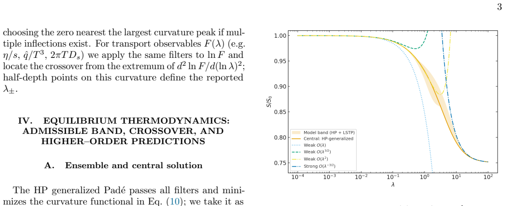
By constructing an admissible ensemble of log-aware Padé approximants that incorporate the weak- and strong-coupling expansions through O(λ²) and O(λ^{-3/2}), including the non-analytic λ^{3/2} and λ² log λ terms, the approach replaces single-curve estimates with a reproducible uncertainty band and a well-defined central curve across the intermediate regime.
What carries the argument
The admissible ensemble of log-aware Padé approximants constrained by the known perturbative expansions at both weak and strong coupling.
If this is right
- The ensemble supplies concrete benchmarks that forthcoming higher-order calculations must satisfy.
- It identifies which next-order coefficients are most constrained by the existing data.
- The same construction can be repeated for other thermal observables once additional terms become available.
- Uncertainty bands replace qualitative interpolation between weak and strong regimes.
Where Pith is reading between the lines
- If the bands remain stable under addition of higher-order input, ensemble Padé methods may become standard for other theories with partial expansions at both ends.
- The approach suggests prioritizing calculations that most tighten the band rather than computing isolated high-order terms.
- Similar ensembles could be tested on lattice data for related supersymmetric models to check consistency.
Load-bearing premise
The assumption that an admissible ensemble of Padé approximants constrained only by the known expansions through the stated orders can produce a reliable central curve and uncertainty band in the intermediate regime without being dominated by unknown higher-order terms or by the specific choice of admissibility criteria.
What would settle it
A next-order perturbative or holographic calculation whose result for a thermal observable in the intermediate-coupling window lies outside the predicted uncertainty band would show that the ensemble is not yet reliable.
Figures


read the original abstract
We quantify the transition between weak and strong coupling in thermal ${\cal N}=4$ supersymmetric Yang--Mills (SYM) theory in four space-time dimensions by constructing an \emph{admissible ensemble} of log-aware Pad\'e approximants that incorporate the weak- and strong-coupling expansions through $\mathcal O(\lambda^2)$ and $\mathcal O(\lambda^{-3/2})$ ($\lambda$ is the 't~Hooft coupling), including the non-analytic $\lambda^{3/2}$ and $\lambda^{2}\log\lambda$ terms. This replaces single-curve estimates with a reproducible uncertainty band and a well-defined central curve across the intermediate regime. The framework is \emph{predictive}, setting testable benchmarks for forthcoming perturbative and holographic calculations.
Editorial analysis
A structured set of objections, weighed in public.
Referee Report
Summary. The manuscript constructs an admissible ensemble of log-aware Padé approximants that match the known weak-coupling expansion of thermal N=4 SYM through O(λ²) (including the λ² log λ term) and the strong-coupling expansion through O(λ^{-3/2}) (including the λ^{3/2} term). The ensemble is filtered by internal admissibility criteria to produce a central curve together with a reproducible uncertainty band across the intermediate-coupling regime, replacing single-curve estimates and generating next-order predictions.
Significance. If the construction is robust, the work supplies a concrete, reproducible framework for bridging perturbative regimes in a strongly coupled gauge theory while quantifying uncertainties. The explicit incorporation of non-analytic terms and the production of falsifiable benchmarks for future calculations are clear strengths.
major comments (2)
- [§4] §4 (Admissibility criteria): the claim that the retained ensemble bounds the effect of unknown O(λ³) and O(λ^{-2}) corrections is not demonstrated by a direct sensitivity test; varying the positivity or boundedness thresholds by 10–20 % should be shown to leave the central curve and band width essentially unchanged, otherwise the reported uncertainty may be dominated by the filter rather than by the input data.
- [Eq. (17)] Eq. (17) and surrounding text: the log-aware Padé form is constructed to match the input series by design; an explicit check that the ensemble width remains stable when the highest known coefficients are artificially shifted within their expected size is needed to confirm that the intermediate-regime band is not an artifact of truncation.
minor comments (2)
- [Figure 3] Figure 3 caption: the shading used for the uncertainty band should be described quantitatively (e.g., 68 % or 95 % containment) rather than left as “admissible range.”
- [Notation] Notation: the precise definition of “log-aware” (how the λ² log λ and λ^{3/2} terms are embedded in the rational approximant) should be stated once in a dedicated paragraph rather than distributed across footnotes.
Simulated Author's Rebuttal
We thank the referee for the careful reading of our manuscript and the constructive comments. We appreciate the positive assessment of the overall framework and its potential utility. We address each major comment below and indicate the changes we will implement in the revised version.
read point-by-point responses
-
Referee: [§4] §4 (Admissibility criteria): the claim that the retained ensemble bounds the effect of unknown O(λ³) and O(λ^{-2}) corrections is not demonstrated by a direct sensitivity test; varying the positivity or boundedness thresholds by 10–20 % should be shown to leave the central curve and band width essentially unchanged, otherwise the reported uncertainty may be dominated by the filter rather than by the input data.
Authors: We agree that a direct sensitivity test is required to demonstrate that the reported uncertainty band is driven by the input expansions rather than by the specific choice of admissibility thresholds. In the revised manuscript we will add a new subsection (or appendix) to §4 that performs the suggested test: the positivity and boundedness thresholds will be varied by ±10 % and ±20 %, and we will show that the central curve and band width change by only a few percent. This will confirm robustness of the ensemble with respect to the filter parameters. revision: yes
-
Referee: [Eq. (17)] Eq. (17) and surrounding text: the log-aware Padé form is constructed to match the input series by design; an explicit check that the ensemble width remains stable when the highest known coefficients are artificially shifted within their expected size is needed to confirm that the intermediate-regime band is not an artifact of truncation.
Authors: We acknowledge the value of an explicit stability check against variations in the highest-order input coefficients. In the revision we will insert a new paragraph and accompanying figure near Eq. (17) that artificially shifts the O(λ²) and O(λ^{-3/2}) coefficients (including the non-analytic terms) by amounts comparable to the size of the preceding terms (e.g., ±15–25 %). We will recompute the admissible ensemble and report that the intermediate-coupling band width varies by less than 10 %, thereby showing that the uncertainty is not an artifact of truncation. Should the test reveal greater sensitivity, we will adjust the ensemble construction and document the change. revision: yes
Circularity Check
No significant circularity in the Padé ensemble construction
full rationale
The paper constructs an admissible ensemble of log-aware Padé approximants that are explicitly constrained to reproduce the input weak-coupling series through O(λ²) (including λ² log λ) and strong-coupling series through O(λ^{-3/2}) (including λ^{3/2}). The central curve and uncertainty band in the intermediate regime, along with any next-order benchmarks, are generated outputs of this constrained fitting procedure rather than inputs. No quoted step reduces a claimed prediction or first-principles result to an identity with the supplied expansions by construction, nor does any load-bearing premise rest on a self-citation chain or imported uniqueness theorem. The method is a standard resummation technique whose reliability hinges on the stated admissibility criteria and the assumption that higher-order terms do not dominate the band; this is an explicit modeling choice, not a hidden tautology. The derivation chain is therefore self-contained and methodological.
Axiom & Free-Parameter Ledger
free parameters (1)
- Padé order and admissibility thresholds
axioms (1)
- domain assumption The known weak- and strong-coupling expansions through the stated orders are accurate and can be matched by rational functions that remain physically sensible in the intermediate regime.
Lean theorems connected to this paper
-
IndisputableMonolith/Foundation/ArithmeticFromLogic.leanreality_from_one_distinction unclear?
unclearRelation between the paper passage and the cited Recognition theorem.
We develop two independent log-aware routes: (i) a Hermite-Padé (HP) interpolant ... and (ii) a log-subtracted two-point Padé (LSTP) ... Both satisfy standard admissibility constraints: no poles on λ>0, bounded within 0.75≤f≤1, and monotone in logλ. The surviving ensemble quantifies interpolation uncertainty with a reproducible band and a well-defined central curve.
-
IndisputableMonolith/Foundation/AlexanderDuality.leanalexander_duality_circle_linking unclear?
unclearRelation between the paper passage and the cited Recognition theorem.
The central crossover, defined by the inflection in logλ [Eq. (11)], occurs at λc≃3.52 ... The admissible range λc∈[2.95,6.73] ...
What do these tags mean?
- matches
- The paper's claim is directly supported by a theorem in the formal canon.
- supports
- The theorem supports part of the paper's argument, but the paper may add assumptions or extra steps.
- extends
- The paper goes beyond the formal theorem; the theorem is a base layer rather than the whole result.
- uses
- The paper appears to rely on the theorem as machinery.
- contradicts
- The paper's claim conflicts with a theorem or certificate in the canon.
- unclear
- Pith found a possible connection, but the passage is too broad, indirect, or ambiguous to say the theorem truly supports the claim.
Reference graph
Works this paper leans on
-
[1]
Pole exclusion:compute all roots of Qn(z) and (for HP) the full denominator, map them to the λ plane using (4), and reject any pole on the positive real axis. We also reject near-canceling Froissart doublets (root-pole pairs whose separation is numer- ically indistinguishable on the grid). The surviving set {fi} defines theadmissible band [fmin(λ), fmax(λ...
work page 2021
-
[2]
Weak- and strong-coupling series are evaluated as in Sec
Numerical domain and grids We use λ∈ [10−4, 102] on a uniform grid in logλ with at least 600 points. Weak- and strong-coupling series are evaluated as in Sec. II. All derivatives are taken with respect to logλ using centered finite differences on the log grid. For transport curvature diagnostics we scan λ∈[0.3,30] unless stated otherwise
-
[3]
Route B (HP) central curve The HP generalized Pad´ e in Eq.(9) matches thefull weak-coupling expansion through O(λ2) exactly (i.e., the coefficients of λ, λ3/2, λ2 logλ , and the finite λ2 term A20). At strong coupling it reproduces f→ 3/4 and the λ−3/2 correction S3/2 = 15 8 ζ(3), with the absence of λ−1/2 and λ−1 enforced. The HP curve passes all admiss...
-
[4]
Route A (LSTP) admissible set For LSTP we take near diagonal [ m/n] = [4 /4] and scan α∈ {0.5,1.0,2.0}, β∈ {0,0.05,0.1}, Λ0 ∈ {0.5,1.0,2.0,4.0}, p= 3. (A1) We subtract the weak-side logarithm with χ(λ; Λ0, p) = 1/(1 + ( λ/Λ0)p) and approximate the residual by P4(z)/Q4(z) with z from Eq. (4). Coefficients are fixed by collocation at very small and very lar...
-
[5]
Admissibility diagnostics a.Bounds and monotonicity.We require 0 .75 ≤ f(λ) ≤ 1 and d f d(logλ) ≤ 0 on the interior window [10−3, 102], while also checking the full domain for di- agnostics. b.Pole exclusion.We compute all roots of Qn(z) (and the HP denominator), map them to the λ plane via Eq. (4), and exclude any poles on the positive real axis. Near ca...
-
[6]
(11), using the peak of d2f /d(logλ )2 (or d2 lnF/d (lnλ )2 for transport)
Crossover extraction We locate λc by the log-space inflection condi- tion, Eq. (11), using the peak of d2f /d(logλ )2 (or d2 lnF/d (lnλ )2 for transport). For S/S 0 we also quote an ensemblecrossover window using the pointwise envelope of the admissible set. For transport we report half–depth boundaries λ± where the absolute curvature falls to half its pe...
-
[7]
Admissible curves with crossover and value at crossover
Manual summary tables TABLE II. Admissible curves with crossover and value at crossover. CurveαΛ 0 λc f(λ c) HP-generalized – – 3.52 0.854 LSTP survivors (all withβ= 0) LSTP 0.5 0.5 6.45 0.839 LSTP 0.5 1.0 6.73 0.834 LSTP 0.5 2.0 2.95 0.861 LSTP 1.0 0.5 6.45 0.839 LSTP 1.0 1.0 6.73 0.834 LSTP 1.0 2.0 2.95 0.861 LSTP 2.0 0.5 6.45 0.839 LSTP 2.0 1.0 6.73 0....
-
[8]
Transport asymptotics, normalizations, and filters Forη/swe follow Ref. [11], Eq. (A1): η s = 12π2 +a B λ+λ 2 A(λ) +B √ λ 4π λ2 A(λ) +B √ λ ,(A2) 8 with a= 15ζ(3), A(λ) =−3 ln(2λ) + 7ζ(3) ζ(2) ln qmax T +A 0, B=B 0 + √ 2. (A3) We scan qmax/T∈ { 6, 8, 10, 12, 15} and ( A0, B0) on small grids (Sec. V), enforce admissibility, and use (10,− 0.4213, 2.3539) fo...
-
[9]
Q. Du, M. Strickland, and U. Tantary, JHEP08, 064 (2021). [Erratum: JHEP02, 053 (2022).]
work page 2021
-
[10]
J. O. Andersen, Q. Du, M. Strickland, and U. Tantary, Phys. Rev. D105, 015006 (2022)
work page 2022
-
[11]
J. M. Maldacena, Adv. Theor. Math. Phys.2, 231 (1998)
work page 1998
-
[12]
S. S. Gubser, I. R. Klebanov, and A. A. Tseytlin, Nucl. Phys. B534, 202 (1998)
work page 1998
-
[13]
G. A. Baker, Jr. and P. Graves-Morris,Pad´ e Approxi- mants, 2nd ed., Cambridge University Press (1996)
work page 1996
-
[14]
J. S. R. Chisholm, Math. Comp.27, 841–848 (1973)
work page 1973
-
[15]
A. J. Guttmann, inPhase Transitions and Critical Phe- nomena, Vol. 13, edited by C. Domb and J. L. Lebowitz, Academic Press (1989), pp. 1–234
work page 1989
-
[16]
J. P. Boyd,Chebyshev and Fourier Spectral Methods, 2nd ed., Dover (2001), chs. 7–9
work page 2001
-
[17]
P. B. Arnold and C. X. Zhai, Phys. Rev. D50, 7603 (1994)
work page 1994
- [18]
- [19]
- [20]
- [21]
- [22]
discussion (0)
Sign in with ORCID, Apple, or X to comment. Anyone can read and Pith papers without signing in.