Recognition: 2 theorem links
· Lean TheoremKinetic-Mamba: Mamba-Assisted Predictions of Stiff Chemical Kinetics
Pith reviewed 2026-05-16 21:37 UTC · model grok-4.3
The pith
Mamba-based neural models predict the full time evolution of stiff chemical kinetics from initial thermochemical states alone.
A machine-rendered reading of the paper's core claim, the machinery that carries it, and where it could break.
Core claim
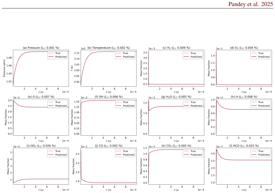
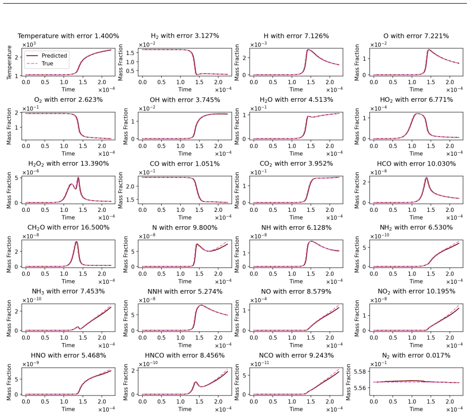
Kinetic-Mamba integrates Mamba sequence models with neural operators to learn the temporal evolution of thermochemical states; the standalone version maps initial conditions directly to future states, the constrained version adds mass-conservation penalties, the regime-informed version deploys separate Mamba models for distinct temperature ranges, and the latent version advances dynamics in a compressed space before lifting back to the physical manifold. Experiments on Syngas and GRI-Mech 3.0 mechanisms confirm high accuracy under both time-decomposition and recursive prediction, including on out-of-distribution initial conditions.
What carries the argument
Mamba sequence model that processes thermochemical state trajectories to predict future states while respecting the underlying reaction manifold.
If this is right
- The standalone Mamba model produces direct state predictions from initial conditions without any differential-equation integration.
- The constrained variant maintains species mass balance throughout the predicted trajectory.
- The regime-informed pair of Mamba models separately captures low- and high-temperature kinetic regimes.
- The latent-space version evolves a compressed representation and reconstructs the full physical state on the manifold.
Where Pith is reading between the lines
- If recursive stability holds, the same architecture could replace stiff integrators in other multi-scale physical systems such as atmospheric chemistry or plasma kinetics.
- Successful out-of-distribution performance suggests the models may generalize to untested reaction mechanisms once trained on a sufficiently diverse set of mechanisms.
- The latent variant implies that dimensionality reduction can be combined with Mamba dynamics to further lower the cost of long-horizon predictions.
Load-bearing premise
The learned Mamba dynamics remain stable and accurate when rolled out recursively over long times and on initial conditions outside the training distribution without accumulating errors from the stiff timescales.
What would settle it
Compare recursive Mamba rollouts against reference stiff-ODE solutions on GRI-Mech 3.0 trajectories started from initial conditions that differ markedly in temperature or composition from the training set; divergence beyond a small tolerance at any time step would falsify the claim.
Figures


read the original abstract
Accurate chemical kinetics modeling is essential for combustion simulations, as it governs the evolution of complex reaction pathways and thermochemical states. In this work, we introduce Kinetic-Mamba, a Mamba-based neural operator framework that integrates the expressive power of neural operators with the efficient temporal modeling capabilities of Mamba architectures. The framework comprises three complementary models: (i) a standalone Mamba model that predicts the time evolution of thermochemical state variables from given initial conditions; (ii) a constrained Mamba model that enforces mass conservation while learning the state dynamics; and (iii) a regime-informed architecture employing two standalone Mamba models to capture dynamics across temperature-dependent regimes. We additionally develop a latent Kinetic-Mamba variant that evolves dynamics in a reduced latent space and reconstructs the full state on the physical manifold. The accuracy and robustness of Kinetic-Mamba was evaluated using both time-decomposition and recursive-prediction strategies. We further assess the extrapolation capabilities of the model on varied out-of-distribution datasets. Computational experiments on Syngas and GRI-Mech 3.0 reaction mechanisms demonstrate that our framework achieves high fidelity in predicting complex kinetic behavior using only the initial conditions of the state variables.
Editorial analysis
A structured set of objections, weighed in public.
Referee Report
Summary. The manuscript introduces Kinetic-Mamba, a Mamba-based neural operator framework for predicting the time evolution of thermochemical states in stiff chemical kinetics. It comprises a standalone Mamba model, a mass-constrained variant enforcing conservation, a regime-informed architecture using two Mamba models for temperature-dependent regimes, and a latent-space version that evolves in reduced space before reconstruction. The models are trained on simulation data and evaluated on Syngas and GRI-Mech 3.0 mechanisms via time-decomposition and recursive-prediction strategies, with additional tests on out-of-distribution initial conditions; the central claim is that these achieve high fidelity using only initial state variables.
Significance. If the recursive predictions prove stable, the framework could supply efficient learned surrogates for stiff ODE integration in combustion modeling, where traditional solvers like CVODE are computationally expensive. The explicit incorporation of mass conservation and regime splitting represents a constructive effort to embed domain knowledge, and the latent-space variant offers a path toward dimensionality reduction. These elements, if quantitatively validated, would strengthen the case for sequence models in multi-timescale physical systems.
major comments (2)
- [Section 4 (recursive-prediction results)] The recursive-prediction evaluation central to the 'only initial conditions' claim lacks any analysis demonstrating that the learned step operator remains contractive on the fast subspace or that local truncation errors remain bounded by the reference stiff integrator over long horizons. Given eigenvalues spanning 6–10 orders of magnitude in stiff kinetics, this omission leaves the robustness claim on autoregressive rollouts unverified.
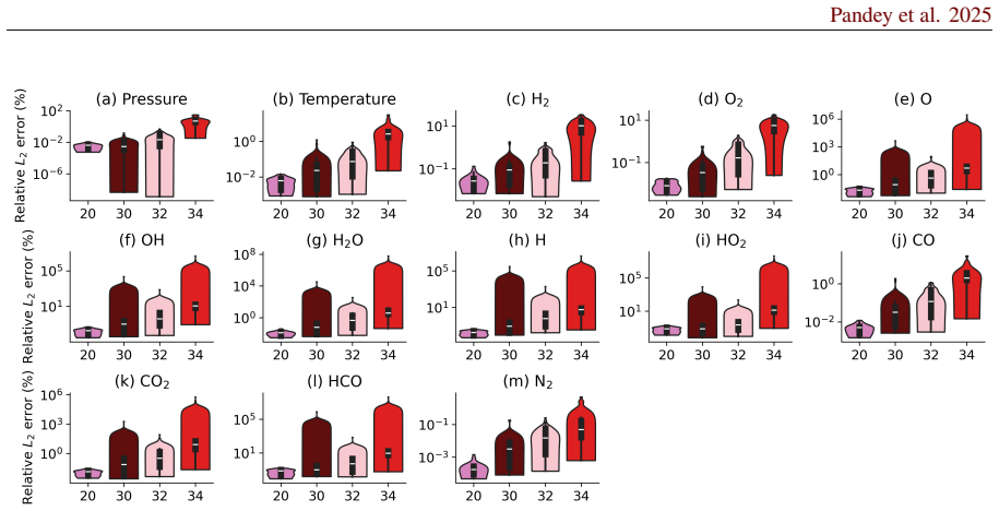
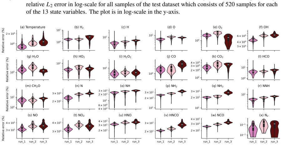
- [Section 4 and associated figures] No quantitative error metrics (e.g., time-averaged L2 norms, maximum pointwise deviations, or integrated error growth rates) or explicit error-bar analysis are supplied for the recursive trajectories on either mechanism, despite the abstract asserting 'high fidelity.' This absence prevents direct assessment of whether predictions remain accurate on slow manifolds after many steps.
minor comments (3)
- [Abstract] The abstract and introduction would benefit from explicit numerical thresholds (e.g., 'relative error below 1%') rather than the qualitative phrase 'high fidelity.'
- [Section 3 (Methods)] Training details (optimizer, learning-rate schedule, batch size, number of epochs, and data-split ratios) are not reported, hindering reproducibility of the supervised learning procedure.
- [Figures in Section 4] Figure captions for prediction plots should include the exact time horizon, number of recursive steps, and reference integrator used for comparison.
Simulated Author's Rebuttal
We thank the referee for the detailed and constructive comments. We address each major point below and will incorporate the suggested enhancements to strengthen the quantitative validation of the recursive predictions.
read point-by-point responses
-
Referee: [Section 4 (recursive-prediction results)] The recursive-prediction evaluation central to the 'only initial conditions' claim lacks any analysis demonstrating that the learned step operator remains contractive on the fast subspace or that local truncation errors remain bounded by the reference stiff integrator over long horizons. Given eigenvalues spanning 6–10 orders of magnitude in stiff kinetics, this omission leaves the robustness claim on autoregressive rollouts unverified.
Authors: We acknowledge the value of a formal stability analysis for stiff systems. Our empirical recursive rollouts on both Syngas and GRI-Mech 3.0 remain stable over the tested horizons without divergence, consistent with the reference integrator. In the revised manuscript we will add a supplementary discussion that estimates the effective Lipschitz constant of the learned step operator (via finite differences on the training trajectories) and compares local truncation error growth against CVODE over multiple characteristic time scales, thereby addressing contractivity on the fast subspace. revision: yes
-
Referee: [Section 4 and associated figures] No quantitative error metrics (e.g., time-averaged L2 norms, maximum pointwise deviations, or integrated error growth rates) or explicit error-bar analysis are supplied for the recursive trajectories on either mechanism, despite the abstract asserting 'high fidelity.' This absence prevents direct assessment of whether predictions remain accurate on slow manifolds after many steps.
Authors: We agree that explicit quantitative metrics would improve clarity. The present figures rely primarily on visual overlay; the revised version will report time-averaged L2 norms, maximum pointwise deviations, and integrated error growth rates for the recursive trajectories on both mechanisms. We will also include error bars derived from an ensemble of out-of-distribution initial conditions to quantify variability on the slow manifolds. revision: yes
Circularity Check
No circularity: standard supervised training on external simulation data
full rationale
The paper trains Mamba-based neural operators on trajectories generated by standard stiff ODE solvers (CVODE/LSODA) for Syngas and GRI-Mech 3.0 mechanisms. Predictions are evaluated via time-decomposition and recursive rollout on held-out and OOD initial conditions. No derivation step equates a claimed prediction to a fitted parameter by construction, no self-citation supplies a uniqueness theorem or ansatz that the central claim depends on, and the architecture is presented as an explicit sequence model without internal redefinition of its outputs. The framework remains a conventional data-driven surrogate whose fidelity claims rest on empirical validation rather than algebraic identity with its training inputs.
Axiom & Free-Parameter Ledger
free parameters (1)
- neural network weights and architecture hyperparameters
axioms (1)
- domain assumption Mamba state-space models can stably approximate the temporal evolution operator of stiff chemical kinetics
Lean theorems connected to this paper
-
IndisputableMonolith/Foundation/RealityFromDistinction.leanreality_from_one_distinction unclear?
unclearRelation between the paper passage and the cited Recognition theorem.
recursive prediction... adaptive time stepping... latent Kinetic-Mamba model
What do these tags mean?
- matches
- The paper's claim is directly supported by a theorem in the formal canon.
- supports
- The theorem supports part of the paper's argument, but the paper may add assumptions or extra steps.
- extends
- The paper goes beyond the formal theorem; the theorem is a base layer rather than the whole result.
- uses
- The paper appears to rely on the theorem as machinery.
- contradicts
- The paper's claim conflicts with a theorem or certificate in the canon.
- unclear
- Pith found a possible connection, but the passage is too broad, indirect, or ambiguous to say the theorem truly supports the claim.
Reference graph
Works this paper leans on
-
[1]
Nedunchezhian Swaminathan and Alessandro Parente.Machine learning and its application to reacting flows: ML and combustion. Springer Nature, 2023
work page 2023
-
[2]
License: Cc by 4.0.IEA: Paris, France, 2023
IEA Global EV Outlook. License: Cc by 4.0.IEA: Paris, France, 2023
work page 2023
-
[3]
S.B. Pope. Computationally efficient implementation of combustion chemistry using in situ adaptive tabulation.Combustion Theory and Modelling, 1(1):41–63, 1997. doi: 10.1080/713665229. URLhttps://doi.org/10.1080/713665229
-
[4]
Robert J Kee, Michael E Coltrin, and Peter Glarborg.Chemically reacting flow: theory and practice. John Wiley & Sons, 2005. 26
work page 2005
-
[5]
CHEMSODE: a stiff ODE solver for the equations of chemical kinetics
Colin J Aro. CHEMSODE: a stiff ODE solver for the equations of chemical kinetics. Computer physics communications, 97(3):304–314, 1996
work page 1996
-
[6]
Colin J Aro. A stiff ODE preconditioner based on newton linearization.Applied numerical mathematics, 21(4):335–352, 1996
work page 1996
-
[7]
Colin J Aro, Douglas A Rotman, and Garry H Rodrigue. A high performance chemical kinetics algorithm for 3-d atmospheric models.International Journal of High Performance Computing Applications, 13(1):3–15, 1999
work page 1999
-
[8]
Donald Dabdub and John H Seinfeld. Extrapolation techniques used in the solution of stiff ODEs associated with chemical kinetics of air quality models.Atmospheric Environment, 29(3):403–410, 1995
work page 1995
-
[9]
Improved traditional rosenbrock–wanner methods for stiff ODEs and DAEs
Joachim Rang. Improved traditional rosenbrock–wanner methods for stiff ODEs and DAEs. Journal of Computational and Applied Mathematics, 286:128–144, 2015. ISSN 0377-0427. doi: https://doi.org/10.1016/j.cam.2015.03.010. URL https://www.sciencedirect. com/science/article/pii/S0377042715001569
-
[10]
Deep learning for scalable chemical kinetics
Alisha J Sharma, Ryan F Johnson, David A Kessler, and Adam Moses. Deep learning for scalable chemical kinetics. InAIAA scitech 2020 forum, page 0181, 2020
work page 2020
-
[11]
Brown, Harbir Antil, Rainald L¨ohner, Fumiya Togashi, and Deepanshu Verma
Thomas S. Brown, Harbir Antil, Rainald L¨ohner, Fumiya Togashi, and Deepanshu Verma. Novel DNNs for Stiff ODEs with Applications to Chemically Reacting Flows. In Heike Jagode, Hartwig Anzt, Hatem Ltaief, and Piotr Luszczek, editors,High Performance Computing, pages 23–39, Cham, 2021. Springer International Publishing. ISBN 978-3- 030-90539-2
work page 2021
-
[12]
Maziar Raissi, Paris Perdikaris, and George E Karniadakis. Physics-informed neural networks: A deep learning framework for solving forward and inverse problems involving nonlinear partial differential equations.Journal of Computational Physics, 378:686–707, 2019
work page 2019
-
[13]
Weiqi Ji, Weilun Qiu, Zhiyu Shi, Shaowu Pan, and Sili Deng. Stiff-PINN: Physics-Informed Neural Network for Stiff Chemical Kinetics.The Journal of Physical Chemistry A, 125(36): 8098–8106, 2021. doi: 10.1021/acs.jpca.1c05102. URL https://doi.org/10.1021/ acs.jpca.1c05102. PMID: 34463510
-
[14]
Matthew Frankel, Mario De Florio, Enrico Schiassi, and Lina Sela. Hybrid chemical and data-driven model for stiff chemical kinetics using a physics-informed neural network. Engineering Proceedings, 69(1):40, 2024
work page 2024
-
[15]
Lu Lu, Pengzhan Jin, Guofei Pang, Zhongqiang Zhang, and George Em Karniadakis. Learning nonlinear operators via DeepONet based on the universal approximation theorem of operators.Nature Machine Intelligence, 3(3):218–229, mar 2021. ISSN 2522-5839. doi: 10.1038/s42256-021-00302-5. URL http://dx.doi.org/10.1038/ s42256-021-00302-5
-
[16]
Fourier Neural Operator for Parametric Partial Differential Equations
Zongyi Li, Nikola Kovachki, Kamyar Azizzadenesheli, Burigede Liu, Kaushik Bhattacharya, Andrew Stuart, and Anima Anandkumar. Fourier neural operator for parametric partial differential equations.arXiv preprint arXiv:2010.08895, 2020
work page internal anchor Pith review Pith/arXiv arXiv 2010
-
[17]
KAN: Kolmogorov-Arnold Networks
Ziming Liu, Yixuan Wang, Sachin Vaidya, Fabian Ruehle, James Halverson, Marin Soljaˇci´c, Thomas Y Hou, and Max Tegmark. KAN: Kolmogorov-arnold networks.arXiv preprint arXiv:2404.19756, 2024
work page internal anchor Pith review Pith/arXiv arXiv 2024
-
[18]
Khemraj Shukla, Juan Diego Toscano, Zhicheng Wang, Zongren Zou, and George Em Karniadakis. A comprehensive and FAIR comparison between MLP and KAN rep- resentations for differential equations and operator networks.Computer Methods in Applied Mechanics and Engineering, 431:117290, 2024. ISSN 0045-7825. doi: https://doi.org/10.1016/j.cma.2024.117290. URLhtt...
-
[19]
Jagtap, Hessam Babaee, Bryan T
Somdatta Goswami, Ameya D. Jagtap, Hessam Babaee, Bryan T. Susi, and George Em Kar- niadakis. Learning stiff chemical kinetics using extended deep neural operators.Computer Methods in Applied Mechanics and Engineering, 419:116674, 2024. ISSN 0045-7825. doi: https://doi.org/10.1016/j.cma.2023.116674. URLhttps://www.sciencedirect.com/ science/article/pii/S0...
-
[20]
Combustion chemistry acceleration with DeepONets.Fuel, 365:131212, 2024
Anuj Kumar and Tarek Echekki. Combustion chemistry acceleration with DeepONets.Fuel, 365:131212, 2024. ISSN 0016-2361. doi: https://doi.org/10.1016/j.fuel.2024.131212. URL https://www.sciencedirect.com/science/article/pii/S0016236124003582
-
[21]
Yuting Weng, Han Li, Hao Zhang, Zhi X. Chen, and Dezhi Zhou. Extended Fourier Neural Operators to learn stiff chemical kinetics under unseen conditions.Combus- tion and Flame, 272:113847, 2025. ISSN 0010-2180. doi: https://doi.org/10.1016/ j.combustflame.2024.113847. URL https://www.sciencedirect.com/science/ article/pii/S001021802400556X
-
[22]
Susi, Hessam Babaee, and George Em Karniadakis
Kamaljyoti Nath, Additi Pandey, Bryan T. Susi, Hessam Babaee, and George Em Karniadakis. AMORE: Adaptive multi-output operator network for stiff chemical kinetics, 2025. URL https://arxiv.org/abs/2510.12999
-
[23]
Efficiently Modeling Long Sequences with Structured State Spaces
Albert Gu, Karan Goel, and Christopher R ´e. Efficiently modeling long sequences with structured state spaces, 2022. URLhttps://arxiv.org/abs/2111.00396
work page internal anchor Pith review Pith/arXiv arXiv 2022
-
[24]
Mamba: Linear-time sequence modeling with selective state spaces
Albert Gu and Tri Dao. Mamba: Linear-time sequence modeling with selective state spaces. arXiv e-prints, pages arXiv–2312, 2023
work page 2023
-
[25]
Zheyuan Hu, Nazanin Ahmadi Daryakenari, Qianli Shen, Kenji Kawaguchi, and George Em Karniadakis. State-space models are accurate and efficient neural operators for dynamical systems.arXiv preprint arXiv:2409.03231, 2024
-
[26]
A Mamba-based foundation model for chemistry
Emilio Vital Brazil, Eduardo Soares, Victor Yukio Shirasuna, Renato Cerqueira, Dmitry Zubarev, and Kristin Schmidt. A Mamba-based foundation model for chemistry. InAI for Accelerated Materials Design-NeurIPS 2024, 2024
work page 2024
-
[27]
Molecular generation with state space sequence models
Anri Lombard, Shane Acton, Ulrich Armel Mbou Sob, and Jan Buys. Molecular generation with state space sequence models. InNeurIPS 2024 Workshop on AI for New Drug Modalities, 2024. URLhttps://openreview.net/forum?id=1ib5oyTQIb
work page 2024
-
[28]
SMILES-Mamba: Chemical mamba foundation models for drug ADMET prediction
Bohao Xu, Yingzhou Lu, Chenhao Li, Ling Yue, Xiao Wang, Nan Hao, Tianfan Fu, and Jim Chen. SMILES-Mamba: Chemical mamba foundation models for drug ADMET prediction. arXiv preprint arXiv:2408.05696, 2024
-
[29]
Bohao Xu, Yingzhou Lu, Yoshitaka Inoue, Namkyeong Lee, Tianfan Fu, and Jintai Chen. Protein-Mamba: Biological Mamba Models for Protein Function Prediction.arXiv preprint arXiv:2409.14617, 2024
-
[30]
GRI 3.0 mechanism.Gas Research Institute, 1999
Gregory P Smith, David M Golden, Michael Frenklach, Nigel W Moriarty, Boris Eiteneer, Mikhail Goldenberg, C Thomas Bowman, Ronald K Hanson, Soonho Song, William C Gardiner Jr, et al. GRI 3.0 mechanism.Gas Research Institute, 1999
work page 1999
-
[31]
David G Goodwin, Harry K Moffat, and Raymond L Speth. Cantera: An Object-oriented Software Toolkit for Chemical Kinetics, Thermodynamics, and Transport Processes. Version 2.3.0.Zenodo, 2017. doi: 10.5281/zenodo.170284
-
[32]
Deepomamba: State-space model for spatio-temporal pde neural operator learning.J
Zheyuan Hu, Qianying Cao, Kenji Kawaguchi, and George Em Karniadakis. Deepomamba: State-space model for spatio-temporal pde neural operator learning.J. Comput. Phys., 540: 114272, 2025. URLhttps://api.semanticscholar.org/CorpusID:280547144
work page 2025
-
[33]
George Karniadakis and Spencer J Sherwin.Spectral/hp element methods for computational fluid dynamics. Oxford University Press, 2005
work page 2005
-
[34]
Adam: A Method for Stochastic Optimization
Diederik P Kingma and Jimmy Ba. Adam: A method for stochastic optimization.arXiv preprint arXiv:1412.6980, 2014. Appendices In the following sections, we shall touch upon several relevant aspects corresponding to the data, implementation and results that we could not include in the main body of the paper. 28 A Range of Data In this section, we report the ...
work page internal anchor Pith review Pith/arXiv arXiv 2014
-
[35]
In the problem corresponding to the Syngas A dataset Section 3.1.1, we observe that the total training time is 161315.47 seconds (44.81 hours) and the prediction time is 2.77 seconds
-
[36]
Moreover, it takes 142.72 seconds to go from the𝑚-dimensional manifold to𝑚+1-dimensional manifold
When we transition to the mass-conserving Kinetic-Mamba framework on the Syngas A dataset Section 3.1.2, we observe that the total training time is 161677.78 seconds (44.91 hours) and the prediction time is 2.74 seconds. Moreover, it takes 142.72 seconds to go from the𝑚-dimensional manifold to𝑚+1-dimensional manifold
-
[37]
When we use the Syngas B dataset with our Kinetic-Mamba framework which takes the ignition regimes into consideration Section 3.1.3, we note that the training time is 12743.51 seconds (3.54 hours) and 185055.27 seconds (51.40 hours) corresponding to the data lying below 𝜏K and above 𝜏K and the prediction times are 0.78 seconds and 4.38 seconds, respectively
-
[38]
When considering the latent Kinetic-Mamba model on the GRI dataset Section 3.1.4, the training time is 45764.18 seconds (12.71 hours) and the prediction time is 0.92 seconds. C Additional Results on Extrapolation and Recursive Prediction We mentioned inflation in the relative 𝐿2 error observed in violin plot Fig. 16 due to small value of the denominator (...
discussion (0)
Sign in with ORCID, Apple, or X to comment. Anyone can read and Pith papers without signing in.