Multi-Distribution Robust Conformal Prediction

Ying Jin; Yuqi Yang

REVIEW 3 major objections 4 minor 1 cited by

Multi-Distribution Robust Conformal Prediction

T0 review · 3 major / 4 minor · reviewed 2026-08-03 · deepseek-v4-flash

Challenge this review Re-run · record.json Download PDF Read on arXiv ↗

Pith's one-line read One prediction set can be valid for every source distribution at once, and max-p aggregation reaches oracle-optimal size in the limit.

desk verdict The max-p aggregation and LP-duality characterization are clean, but Theorem 3's proof has a real gap: the uniqueness of the α-quantile is asserted without justification, so the asymptotic optimality claim likely needs extra assumptions. read the letter →

arxiv 2601.02998 v2 pith:G7JMC3BO submitted 2026-01-06 cs.LG stat.MEstat.ML

Yuqi Yang , Ying Jin This is my paper · ORCID

classification cs.LGstat.MEstat.ML

keywords conformalpredictionmultipledistributionsuniformcoveragemax-paggregationdistributionallyrobustsubpopulationshiftgroup-conditionalvaliditysetefficiency

verification ladder T0 review T1 audit T2 compute T3 formal

The pith

A machine-rendered reading of the paper's core claim, the machinery that carries it, and where it could break.

The reading

The paper studies how to build one prediction set that remains valid no matter which of several known source distributions the test point comes from — a setup that appears when protecting against subpopulation shift, when group labels are unavailable, or when data come from several hospitals or regions. Its central proposal, max-p aggregation, computes a conformal p-value for each source and takes their maximum, which is equivalent to taking the union of per-source prediction sets and immediately yields finite-sample coverage for every source and every mixture of them. The paper further claims that this aggregation is not wasteful: there is a single shared score — a weighted sum of the sources' conditional label densities, with covariate-dependent weights — such that max-p aggregation converges to the smallest set that is uniformly valid, and at least one source's coverage is exactly at the nominal level. If correct, the practitioner gets one set valid everywhere, with size approaching the oracle optimum, rather than an over-conservative union.

What carries the argument

The max-p aggregation rule p(y) = max_k p^{(k)}(y), inverted to C(x) = {y : p(y) ≥ α}, equals the union of the per-source conformal sets. The theoretical driver is the shared score h_λ(x,y) = Σ_k λ_k(x) f_k(y|x), with the dual multipliers λ* from a size-minimization program. It encodes which sources constrain the set locally, and its superlevel set {h* ≥ 1} is the oracle-optimal uniformly valid set.

What would settle it

Take K=2 sources with known overlapping densities and compute the exact dual weights. If, with n growing, the size of the max-p aggregated set does not converge to the size of {y: h*(x,y) ≥ 1} up to the boundary, the asymptotic optimality claim fails; equally, if the worst-case source coverage stays strictly above 1−α with no downward trend as n grows, the tightness claim fails.

Watch

Extended reading notes

Core claim

Fix a covariate x. The oracle-optimal set under uniform coverage has the form {y: Σ_k λ_k*(x) f_k(y|x) > 1} up to boundary randomization, where the multipliers λ_k*(x) mark which sources are hardest to cover at x (a positive multiplier means that source's coverage constraint is active). The paper proves that max-p aggregation built from consistent estimates of these densities and multipliers converges to this oracle set, and that the final set achieves exact 1−α coverage for at least one source. The finite-sample validity of the union is distribution-free and does not depend on how the per-source scores were trained.

Load-bearing premise

The coverage guarantee itself only needs split conformal calibration, but the efficiency and tightness claims require that each source's conditional label density and the optimal weights are estimated consistently — if those estimates are poor, the set remains valid but can be larger than necessary.

Editorial extensions

If this is right

A practitioner can return a single prediction set with guaranteed coverage for every source or any mixture of sources, without observing the source label at test time.
Efficiency can match single-source conformal sets: with learned scores, the union shrinks toward the oracle set rather than inflating.
Worst-case coverage is tight: at least one source is covered at exactly 1−α asymptotically, so the method is not needlessly conservative.
The framework covers subpopulation shift and fairness without protected group labels, since any mixture of sources inherits the guarantee.
In regression, the MDCP set is a union of at most K intervals, giving an efficient grid-search implementation.

Reading between the lines

Editorial extensions of the paper, not claims the author makes directly.

The dual weights λ_k(x) are an interpretable by-product: they identify, at each x, which source is hardest to cover; one could use them as a diagnostic for where a source is under-served by the model.
A natural extension is to replace the density-based score with quantile or interval-preserving scores so the final set in regression is always an interval; the paper's own discussion suggests this as an open question.
Because finite-sample validity is score-agnostic but efficiency depends on density estimation, a testable practical prediction is that MDCP's size advantage over naive union grows as the per-source density estimates improve (more data per source).
The framework assumes the test point comes from one of the known sources or their mixture; applying it to a genuinely new environment is outside the guarantee and would require additional handling of novel groups.

Share X Bluesky LinkedIn Reddit HN

Editorial analysis

A structured set of objections, weighed in public.

Desk editor's note, referee report, and a circularity audit.

Desk Editor's Note

read the letter

The core of the paper is solid. The max-p aggregation scheme is simple, and the finite-sample uniform coverage guarantee in Theorem 1 is correct and unconditional. The dual characterization in Theorem 2—the optimal set as a mixture-of-densities superlevel set, with the λ_k(x) weights identifying the active sources—is clean and genuinely useful. The algorithm is sensible, and the experiments are extensive; the code release helps. This is a serious paper with real content.

The soft spot is Theorem 3, and it is not minor. The proof in Appendix B.4 claims that for an active source with λ_k(x)>0, α lies in the jump [F_k(1−), F_k(1)] and therefore the generalized α-quantile is unique and equals 1. That inference is invalid. α belonging to the quantile set does not imply uniqueness. If the CDF F_k is flat at level α on an interval [a,1) with a<1—which can happen when h* takes values with a gap in its range, for instance with piecewise densities—then every q∈[a,1] is an α-quantile. The empirical quantile then converges to the lower endpoint a, not to 1, and the max-p set converges to {h*>a}, adding the positive-measure region {a

This is a load-bearing flaw in the paper's main asymptotic claim, but it is repairable. The authors need to either add assumptions guaranteeing uniqueness of the α-quantile for at least one active source and no quantiles below 1 (e.g., no flat segments at the α-level, or a condition like the CDF being strictly increasing through α), or substantially rework the proof. Without that, the 'optimal and tight' claim goes beyond what is proven.

Two smaller points: Theorem 9's proof is delegated to an overlapping-author paper (Jin et al. 2022); that should be made self-contained or the conditions verified. And the Gaussian working model in regression is a misspecification risk—coverage holds, but the efficiency story depends on it; the paper acknowledges this implicitly via the log transform in MEPS, but it should be stated in the main text.

Verdict: this paper deserves a serious referee and will likely be accepted after revision. The finite-sample validity and the dual characterization are worth keeping; the asymptotic optimality needs fixing before I'd cite it as a result.

Referee Report

3 major / 4 minor

Summary. The paper proposes Multi-Distribution Conformal Prediction (MDCP): combine per-source conformal p-values by taking their maximum, and invert the max-p p-value to obtain a prediction set. Theorem 1 shows this aggregation is the union of single-source conformal sets and provides finite-sample uniform coverage for any conformity scores. For efficiency, the paper studies population-level size-minimization programs under uniform coverage (Theorems 2 and 10), characterizes the oracle-optimal set as a superlevel set of a shared score h*(x,y)=Σ_k λ_k*(x) f_k(y|x), and claims in Theorem 3 that max-p aggregation with consistent estimates of this score is asymptotically optimal and tight up to the boundary {h*=1}. The practical algorithm learns λ(·) by empirical dual objective (Theorem 9), with instantiations for classification and regression, supported by simulations and three real-data applications.

Significance. The finite-sample uniform-coverage result (Theorem 1) is clean, useful, and score-agnostic, and the LP-duality characterization of an oracle-optimal set is a valuable conceptual contribution. If the asymptotic optimality claim is made rigorous, the paper gives a principled way to design shared conformity scores for multi-distribution conformal prediction without group labels, with substantial potential application to fairness and subpopulation shift. The experiments are extensive and the code is available. However, the proof of the central asymptotic-optimality theorem has a gap, and the score-learning theorem rests on an undefined and potentially circular assumption; these issues currently prevent the theoretical contribution from being fully accepted as written.

major comments (3)

[Appendix B.4, proof of Theorem 3] The proof asserts, for an active source k, that α∈[F_k(1−),F_k(1)] implies 'the generalized α-quantile is unique and equals 1.' This implication is false: if F_k is flat at level α on an interval [a,1) (e.g., h* takes the value a on a set of P_k-probability α and takes no values in (a,1)), then every q∈[a,1] is a generalized α-quantile, and 1 is not unique. Consequently, the conclusion q̂_{min,α}→1 and the bound ρ(Ĉ^{(n)} △ {h*≥1}) ≤ ρ(T) are not established by the given argument. A correct proof must either add an explicit no-flat-region/uniqueness assumption or show that any limit point of the randomized inf-quantile above 1 corresponds to a ρ-null region {1<h*<q}. The concrete counterexample circulated with the paper is not itself convincing as a feasibility counterexample as written—the second source has zero coverage in the proposed oracle set—but the proof gap is real and load-bear
[Section 4.1, Assumptions 7–8 and proof of Theorem 9] Assumption 7 references λ̄*(x), but this object is never defined in the main text or in the proof of Theorem 9. If λ̄* is the population minimizer with the true p_pool, the assumption is close to vacuous; if it is a different quantity, the triangle inequality '∥λ̂−λ*∥ ≤ ∥λ̂−λ̄*∥ + ∥λ̄*−λ*∥' is not justified, and the assumed rate in Assumption 7 appears to contain the very convergence the theorem is meant to deliver. Moreover, Assumption 8 is asserted without verification for the sieve examples. As written, Theorem 9 does not provide a self-contained derivation of consistency of λ̂ to the dual solution. Please define λ̄*, state precisely which convergence is being assumed, and either verify or substantially weaken Assumptions 7–8.
[Sections 4.3 and 6.3 (regression implementation)] Theorem 3 requires sup-consistent estimation of each true conditional density f_k(y|x). The regression algorithm instead uses a heteroskedastic Gaussian working model f̂_k(y|x)=N(y; μ̂_k(x), σ̂_k^2(x)). On the MEPS data the authors themselves apply a log transform because the raw label density is visibly skewed, showing that the working density is misspecified. Under misspecification ĥ does not converge to h*, so the claimed asymptotic efficiency optimality is not in force for these real-data comparisons (the finite-sample coverage guarantee from Theorem 1 is unaffected). The paper should either provide a misspecification analysis, prove optimality within the Gaussian working model, or explicitly label the real-data efficiency claims as heuristic.

minor comments (4)

[Theorem 3 statement] The statement uses a deterministic-looking limsup of ρ(Ĉ^{(n)} △ {h*≥1}) after the proof has only established convergence in probability of the relevant quantities. The mode of convergence (in probability, almost sure, or along subsequences) should be made explicit and the proof adjusted accordingly.
[Section 4.1, Assumption 8] The notation for function classes is inconsistent: Assumption 8 refers to θ*∈(Λ_c^p)^K, while the preceding text defines Λ_{c,+}^p and Θ=(Λ_{c,+}^p)^K. Please clarify whether nonnegativity is enforced in the Hölder class or handled separately.
[Appendix B.4, Definition 13] The randomized empirical quantile uses a '+1' in the tie term, which differs from the more common convention. The effect of this choice on the limit of the quantile in the presence of atoms should be stated explicitly, since it is relevant to the proof of Theorem 3.
[Section 6.1 / references] The MEPS19 and MEPS20 references appear to point to the same data-file URL; please check that both panels are cited with their correct identifiers.

Circularity Check

1 steps flagged · score 2.0 of 10

No significant circularity; central validity and optimality derivations are self-contained, with only a minor self-citation for sieve convergence rates.

other [Section 4.1 (Theorem 9) and Appendix B.6]
"Similar to Jin et al. [2022, Theorem 1], we can show that the solution (10) is close to λ* once p̂pool is accurate."

The bridge from the fitted score to asymptotic optimality requires convergence λ̂→λ*. The paper's proof of this rate is explicitly delegated to a theorem of a prior preprint co-authored by the present second author — 'Similar to Jin et al. [2022, Theorem 1]' — rather than re-derived from the current assumptions. This is a self-citation chain in a supporting role: if the cited theorem were set aside, Theorem 9 would have no independent derivation in this manuscript. It is not a full circularity because the finite-sample coverage guarantee (Theorem 1) is calibration-based and does not rely on λ̂, and the oracle-optimal form is derived from the LP dual rather than from the fitted model.

full rationale

The central finite-sample uniform coverage (Theorem 1) is a direct split-conformal argument (union of per-source sets), holding for arbitrary scores and any mixture of sources; it is not an input being rediscovered. The optimality result (Theorem 2) is a standalone LP/dual derivation with explicit KKT complementary slackness; Theorem 3 is a conditional statement: if density estimators and dual-weight estimators are consistent, the max-p set converges to the oracle set. The learned λ̂ enters only through an ERM/dual objective whose convergence (Theorem 9) is stated under explicit assumptions (Assumptions 7 and 8). The residual self-citation is to the authors' own prior sieve-rate theorem in the proof of Theorem 9; it is supporting, not load-bearing for validity, and is not a prediction that reduces to a fitted constant. The skeptically flagged issue in Appendix B.4 (uniqueness of the α-quantile on flat regions) is a mathematical correctness/tightness concern, not circularity; it does not raise the circularity score.

Assumptions & free parameters 3 free parameters · 6 assumptions · 1 invented entities

The method's load-bearing fitted components are the per-source density models and the dual weights λ(x); validity does not depend on them, but the efficiency and tightness claims do. The axioms are standard LP duality, standard concentration tools, the problem-domain restriction to the source convex hull, and two regularity conditions (7-8) specific to the proof of Theorem 9. No physical entities are invented.

free parameters (3)

Dual multiplier functions λ_k(x) = ERM fit: cubic B-spline degree 3, 5 knots (simulations) or 2-layer NN width 4 (FMoW/PovertyMap/MEPS)
The theory requires the population LP dual maximizer λ*(x) (Theorem 2); in practice λ is fit on training data via objective (13). Consistency requires Assumption 7 and Theorem 9, and the practical parameterizations do not implement the sieve rate J_n ≍ (n/log n)^{1/(2p+d)}.
Per-source conditional density models f̂_k(y|x) and p̂_pool = Gradient-boosting classifiers (classification); gradient-boosting μ_k(x), σ_k(x) under a Gaussian working model (regress
The shared score h = Σ λ_k f̂_k depends on these fits; Theorem 3's optimality requires sup|f̂_k−f_k| → 0. These are fitted to training folds, and efficiency (not validity) is tied to their accuracy.
Misc hyperparameters: knots (5), NN width (4), PCA dim (16), grid M, penalty γ = 5; 4; 16; M≈100; γ ∈ {0,0.001,...,1000} chosen via mimic split
Chosen by hand; the γ ablation shows negligible effect (suggesting stability), but these choices affect reported set sizes and are not derived from theory.

assumptions (6)

standard math Strong LP duality (Slater's condition) for the coverage LPs in Theorems 2 and 10 (C(x)=Y is strictly feasible).
Used to obtain the threshold form {h>1} and complementary slackness; standard and valid.
standard math Standard empirical-process/concentration tools: DKW inequality, Lévy-distance continuity of quantiles (Appendix B.4).
Used in Theorem 3 to show min-quantile convergence; standard probability theory.
domain assumption Test distribution is one of the K sources or a fixed mixture of them (eq. 1); per-source data are i.i.d.
The entire guarantee is for the convex hull of the source distributions; new environments are out of scope (also acknowledged in Discussion).
domain assumption Each source has covariate density r_k w.r.t. ν and conditional density f_k(y|x) w.r.t. a common reference μ; ν(X), μ(Y) finite (§3.1).
Needed for the pointwise LP and for comparing densities across sources on a common measure.
domain assumption Regression working model Y = μ_k(x) + σ_k(x)ε with ε ~ N(0,1) per source; sup|f̂_k−f_k| → 0 and sup‖λ̂−λ*‖ → 0 (Theorem 3).
The efficiency/optimality result is conditional on consistent density estimation; the Gaussian working model is a practical instantiation that can be misspecified.
ad hoc to paper Assumption 7: ∥λ*−λ̄*∥ = O_P(∥p̂_pool−p_pool∥), and Assumption 8: η-strong convexity of the ERM loss at λ̄*(x).
These conditions are tailored to make Theorem 9's proof go through; Assumption 7 in particular partly assumes the desired convergence transfer.

invented entities (1)

Dual multiplier functions λ_k(x) (softplus parameterization) independent evidence
purpose: Locally weight per-source conditional densities to define the shared optimal score h(x,y)=Σ_k λ_k(x) f_k(y|x), whose superlevel set is the size-optimal uniformly-valid set.
λ is estimated from data via the empirical dual objective (13), not postulated; the theory characterizes the population optimum, and the held-out experiments provide falsifiable coverage/size evidence. It is a functional parameter of the method, not a physical entity.

how reviews work

0 comments

Cite this review

Pith. "Pith review of Multi-Distribution Robust Conformal Prediction." pith.science (2026). https://pith.science/paper/G7JMC3BO

@misc{pith2026260102998,
  author       = {Pith},
  title        = {Pith review of: Multi-Distribution Robust Conformal Prediction},
  year         = {2026},
  howpublished = {\url{https://pith.science/paper/G7JMC3BO}},
  note         = {Machine review of arXiv:2601.02998}
}

read the original abstract

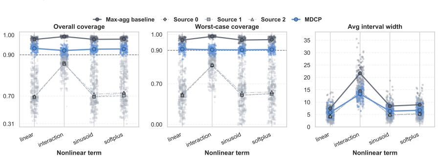
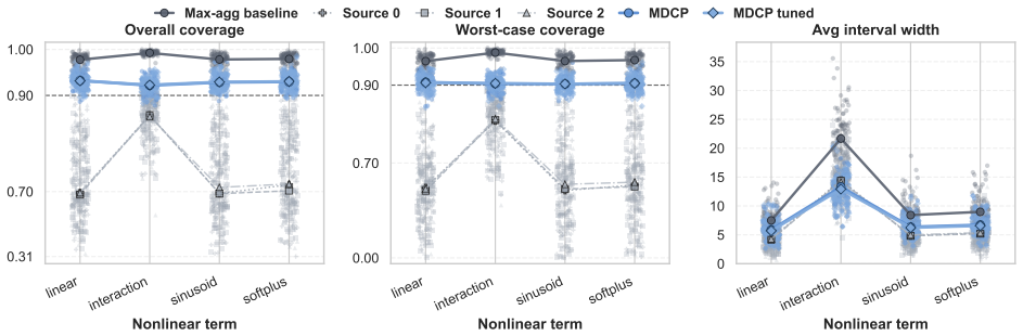
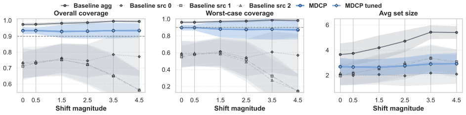
In many fairness and distribution robustness problems, one has access to labeled data from multiple source distributions yet the test data may come from an arbitrary member or a mixture of them. We study the problem of constructing a conformal prediction set that is uniformly valid across multiple, heterogeneous distributions, in the sense that no matter which distribution the test point is from, the coverage of the prediction set is guaranteed to exceed a pre-specified level. We first propose a max-p aggregation scheme that delivers finite-sample, multi-distribution coverage given any conformity scores associated with each distribution. Upon studying several efficiency optimization programs subject to uniform coverage, we prove the optimality and tightness of our aggregation scheme, and propose a general algorithm to learn conformity scores that lead to efficient prediction sets after the aggregation under standard conditions. We discuss how our framework relates to group-wise distributionally robust optimization, sub-population shift, fairness, and multi-source learning. In synthetic and real-data experiments, our method delivers valid worst-case coverage across multiple distributions while greatly reducing the set size compared with naively applying max-p aggregation to single-source conformity scores, and can be comparable in size to single-source prediction sets with popular, standard conformity scores.

Figures

Figures reproduced from arXiv: 2601.02998 by the authors.

**Figure 1.** Prediction sets with uniform coverage need to balance the coverage across multiple distributions. (a) When one distribution has heavier tails, a valid prediction set Cˆ(X) may coincide with the larger one Cˆ1(X). (b) When two distributions partially overlap, a uniformly valid prediction set Cˆ(X) sits in between two distributions and is longer than single-source sets Cˆ1(X) and Cˆ2(X). (c) MDCP achieves uniform cove… view at source ↗

**Figure 2.** Performance of MDCP and baselines in the classification Linear experiments, where the bars represent the result of each method averaged over N = 100 runs, and the dots represent the result in each run. Left: coverage over all test data. Middle: worst-case coverage over single-source test data. Right: average set size over all test data. Simulation results [PITH_FULL_IMAGE:figures/full_fig_p013_2.png] view at source ↗

**Figure 3.** presents the results in the Nonlinear settings. While single-source calibration severely undercovers, MDCP maintains tight worst-case coverage across all settings. MDCP again produces much smaller prediction sets relative to Baseline-agg. Notably, in the softplus setting, MDCP achieves even smaller set sizes than single-source sets, showing the benefits of both max-p aggregation and efficiency optimization: MDCP ad… view at source ↗

Figures from the paper (20 more)

**Figure 4.** Figure 4: Performance of MDCP and baselines in the classification Temperature experiments. The x-axis is the temperature parameter τ . Each line shows the results of a method averaged over N = 100 runs, with shaded ±1 standard deviation across runs. Left: coverage over all test …

**Figure 5.** Figure 5: Evaluation with regression Linear suites; details are otherwise the same as [PITH_FULL_IMAGE:figures/full_fig_p015_5.png]

**Figure 6.** Figure 6: Evaluation with regression Nonlinear suites; details are otherwise the same as in [PITH_FULL_IMAGE:figures/full_fig_p015_6.png]

**Figure 7.** Figure 7: Evaluation with regression Temperature suites; details are otherwise the same as in [PITH_FULL_IMAGE:figures/full_fig_p016_7.png]

**Figure 8.** Figure 8: Performance of MDCP, Baseline-agg, and Baseline-src-k with each source region on the FMoW dataset across six sources: Africa, Americas, Asia, Europe, Oceania, and Other. The bars show the average results over N = 100 runs, and the dots show the result in each run. Left…

**Figure 9.** Figure 9: Results of MDCP and baselines in the PovertyMap dataset. [PITH_FULL_IMAGE:figures/full_fig_p018_9.png]

**Figure 10.** Figure 10: Results of MDCP and baselines in the MEPS dataset evaluation across three panels and two sensitive groups (sources), white and non-white. The bars show results averaged over N = 100 runs, and the dots show single-run results. Each row corresponds to one panel, and eac…

**Figure 11.** Figure 11: Evaluation on the classification Linear suites, where MDCP with data-driven γ ∗ is labeled as “MDCP tuned”. All other experimental settings are identical to those in [PITH_FULL_IMAGE:figures/full_fig_p038_11.png]

**Figure 12.** Figure 12: Evaluation on the classification Nonlinear suites. Experimental settings are identical to [PITH_FULL_IMAGE:figures/full_fig_p039_12.png]

**Figure 13.** Figure 13: Evaluation on the classification Temperature suites. Experimental settings are identical to [PITH_FULL_IMAGE:figures/full_fig_p039_13.png]

**Figure 14.** Figure 14: Results on the regression Linear suites, where MDCP with the selected penalty strength parameter γ ∗ appears as “MDCP tuned”. All other experimental settings match those in [PITH_FULL_IMAGE:figures/full_fig_p039_14.png]

**Figure 15.** Figure 15: Results on the regression Nonlinear suites Experimental settings match those in [PITH_FULL_IMAGE:figures/full_fig_p040_15.png]

**Figure 16.** Figure 16: Results on the regression Temperature suites. Experimental settings match those in [PITH_FULL_IMAGE:figures/full_fig_p040_16.png]

**Figure 17.** Figure 17: Results on the FMoW data, using the algorithmic procedure described in Section 6.1. MDCP and tuned MDCP produce closely aligned performance in this case. Baseline agg RuralUrbanMDCP MDCP tuned Method 0.65 0.90 0.98 Overall coverage Baseline agg RuralUrbanMDCP MDCP tun…

**Figure 18.** Figure 18: Results on the PovertyMap data, using the algorithmic procedure described in Section 6.2. Introducing the parameter γ increases the variability of efficiency. D.2 Additional simulations in covariate shift settings To evaluate MDCP in regimes where covariate shift cont…

**Figure 19.** Figure 19: Results on the MEPS data, using the algorithmic procedure described in Section 6.3. Introducing γ provides a modest improvement to tuned MDCP, offering slightly better efficiency on this highly skewed dataset. (i). Baseline-src-k: The standard conformal prediction set…

**Figure 20.** Figure 20: Performance of MDCP and baselines in the classification Covariate-shift experiments. The x-axis is the covariate-shift magnitude δX, which determines P (k) X separation while keeping P(Y | X) fixed. Each line reports the mean over N = 100 runs, and the shaded region i…

**Figure 21.** Figure 21: Performance of MDCP and baselines in the classification Covariate-and-concept-shift experiments. The x-axis is the covariate shift magnitude δX, with both P (k) X and P (k) (Y | X) varying across sources. Each line reports the mean over N = 100 runs, and the shaded re…

**Figure 22.** Figure 22: Evaluation with regression Covariate-shift suites; details are otherwise the same as in [PITH_FULL_IMAGE:figures/full_fig_p044_22.png]

**Figure 23.** Figure 23: Evaluation with regression Covariate-and-concept-shift suites; details are otherwise the same as in [PITH_FULL_IMAGE:figures/full_fig_p044_23.png]

Discussion (0). Continue with ORCID to comment.

Forward citations

Cited by 1 Pith paper

Reviewed papers in the Pith corpus that reference this work. Sorted by Pith novelty score. Full citation record

Conformalized Large Language Models under Configuration Shift
cs.LG 2026-08 conditional novelty 7.0 of 10

Configuration shift (prompt, temperature, quantization) moves nonconformity score distributions and drives conformal coverage below target; bounds, diagnostics, and mitigations are provided.

Reference graph

Works this paper leans on

4 extracted references · 2 linked inside Pith · cited by 1 Pith paper

[1938]

Kaiming He, Xiangyu Zhang, Shaoqing Ren, and Jian Sun

PMLR, 2018. Kaiming He, Xiangyu Zhang, Shaoqing Ren, and Jian Sun. Deep residual learning for image recognition,

2018
[2009]

Rina Foygel Barber, Emmanuel J Candes, Aaditya Ramdas, and Ryan J Tibshirani

doi: 10.1109/CVPR.2009.5206848. Rina Foygel Barber, Emmanuel J Candes, Aaditya Ramdas, and Ryan J Tibshirani. The limits of distribution-free conditional predictive inference.Information and Inference: A Journal of the IMA, 10(2):455–482, 2021. Yarin Gal et al. Uncertainty in deep learning. 2016. Stuart Geman and Chii-Ruey Hwang. Nonparametric maximum lik...

arXiv 2009
[2015]

Gao Huang, Zhuang Liu, Laurens van der Maaten, and Kilian Q

URLhttps://arxiv.org/abs/1512.03385. Gao Huang, Zhuang Liu, Laurens van der Maaten, and Kilian Q. Weinberger. Densely connected convolu- tional networks, 2018. URLhttps://arxiv.org/abs/1608.06993. Kexin Huang, Ying Jin, Emmanuel Candes, and Jure Leskovec. Uncertainty quantification over graph with conformalized graph neural networks.Advances in Neural Inf...

arXiv 2018
[7501]

measurable

PMLR, 2021. 22 MEPS19. Medical expenditure panel survey, panel 19.https://meps.ahrq.gov/mepsweb/data_stats/ download_data_files_detail.jsp?cboPufNumber=HC-181. Accessed: Oct, 2025. MEPS20. Medical expenditure panel survey, panel 20.https://meps.ahrq.gov/mepsweb/data_stats/ download_data_files_detail.jsp?cboPufNumber=HC-181. Accessed: Oct, 2025. MEPS21. Me...

arXiv 2021

Pith tools

Reviewed August 3, 2026 · model on record in the stance chip above.

[1] [1938]

Kaiming He, Xiangyu Zhang, Shaoqing Ren, and Jian Sun

PMLR, 2018. Kaiming He, Xiangyu Zhang, Shaoqing Ren, and Jian Sun. Deep residual learning for image recognition,

2018

[2] [2009]

Rina Foygel Barber, Emmanuel J Candes, Aaditya Ramdas, and Ryan J Tibshirani

doi: 10.1109/CVPR.2009.5206848. Rina Foygel Barber, Emmanuel J Candes, Aaditya Ramdas, and Ryan J Tibshirani. The limits of distribution-free conditional predictive inference.Information and Inference: A Journal of the IMA, 10(2):455–482, 2021. Yarin Gal et al. Uncertainty in deep learning. 2016. Stuart Geman and Chii-Ruey Hwang. Nonparametric maximum lik...

arXiv 2009

[3] [2015]

Gao Huang, Zhuang Liu, Laurens van der Maaten, and Kilian Q

URLhttps://arxiv.org/abs/1512.03385. Gao Huang, Zhuang Liu, Laurens van der Maaten, and Kilian Q. Weinberger. Densely connected convolu- tional networks, 2018. URLhttps://arxiv.org/abs/1608.06993. Kexin Huang, Ying Jin, Emmanuel Candes, and Jure Leskovec. Uncertainty quantification over graph with conformalized graph neural networks.Advances in Neural Inf...

arXiv 2018

[4] [7501]

measurable

PMLR, 2021. 22 MEPS19. Medical expenditure panel survey, panel 19.https://meps.ahrq.gov/mepsweb/data_stats/ download_data_files_detail.jsp?cboPufNumber=HC-181. Accessed: Oct, 2025. MEPS20. Medical expenditure panel survey, panel 20.https://meps.ahrq.gov/mepsweb/data_stats/ download_data_files_detail.jsp?cboPufNumber=HC-181. Accessed: Oct, 2025. MEPS21. Me...

arXiv 2021