Replacing Tunable Parameters in Weather and Climate Models with State-Dependent Functions using Reinforcement Learning
Pith reviewed 2026-05-16 16:30 UTC · model grok-4.3
The pith
Reinforcement learning learns state-dependent corrections to replace fixed tunable parameters in idealized weather and climate models.
A machine-rendered reading of the paper's core claim, the machinery that carries it, and where it could break.
Core claim
Reinforcement learning agents can learn skilful state-dependent parametrization components in idealized settings, with TQC, DDPG and TD3 showing highest skill and stable convergence; single-agent control outperforms static tuning in the EBM especially in tropical and mid-latitude bands, while federated multi-agent DDPG with frequent aggregation yields the lowest area-weighted RMSE, and the learned corrections prove physically meaningful by modulating radiative parameters, lapse rates and heating increments to limit drift.
What carries the argument
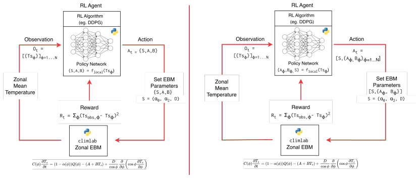
Reinforcement learning agents that map current model state to updates of parametrization parameters, trained to minimize diagnostics such as area-weighted RMSE in single-agent and federated multi-agent settings.
If this is right
- State-dependent corrections reduce meridional temperature biases more effectively than fixed parameters in the energy-balance model.
- Federated multi-agent RL enables specialized regional control and faster convergence than a single global agent.
- The learned adjustments adjust lapse rates and heating increments in ways that match observed vertical and meridional error patterns.
- Online learning replaces offline tuning of fixed coefficients, potentially allowing models to adapt during integration.
Where Pith is reading between the lines
- If the approach scales, models could continuously adjust sub-grid schemes in response to changing large-scale conditions such as altered circulation regimes.
- Multi-agent federated training may offer a practical route for regional specialization without separate offline tuning campaigns for each domain.
- The same RL machinery could be tested on additional parametrization targets such as cloud microphysics or boundary-layer mixing once stability issues are addressed.
Load-bearing premise
Performance improvements seen in the three simple idealized testbeds will carry over to full-complexity weather and climate models without introducing numerical instabilities or unphysical drift.
What would settle it
Apply the trained RL policies inside a full global climate model and check whether area-weighted RMSE decreases while long-term temperature and energy drifts remain within acceptable bounds and no new instabilities appear.
Figures


read the original abstract
Weather and climate models rely on parametrisations to represent unresolved sub-grid processes. Traditional schemes rely on fixed coefficients that are weakly constrained and tuned offline, contributing to persistent biases that limit their ability to adapt to underlying physics. This study presents a framework that learns components of parametrisation schemes online as a function of the evolving model state using reinforcement learning (RL) and evaluates RL-driven parameter updates across idealised testbeds spanning a simple climate bias correction (SCBC), a radiative-convective equilibrium (RCE), and a zonal mean energy balance model (EBM) with single-agent and federated multi-agent settings. Across nine RL algorithms, Truncated Quantile Critics (TQC), Deep Deterministic Policy Gradient (DDPG), and Twin Delayed DDPG (TD3) achieved the highest skill and stable convergence, with performance assessed against a static baseline using area-weighted RMSE, temperature and pressure-level diagnostics. For the EBM, single-agent RL outperformed static parameter tuning with the strongest gains in tropical and mid-latitude bands, while federated RL on multi-agent setups enabled specialised control and faster convergence, with a six-agent DDPG configuration using frequent aggregation yielding the lowest area-weighted RMSE across the tropics and mid-latitudes. The learnt corrections were also physically meaningful as agents modulated EBM radiative parameters to reduce meridional biases, adjusted RCE lapse rates to match vertical temperature errors, and stabilised heating increments to limit drift. Overall, results show that RL can learn skilful state-dependent parametrisation components in idealised settings, offering a scalable pathway for online learning within numerical models and a starting point for evaluation in weather and climate models.
Editorial analysis
A structured set of objections, weighed in public.
Referee Report
Summary. The manuscript proposes replacing fixed tunable parameters in weather and climate model parametrizations with state-dependent functions learned online via reinforcement learning. It evaluates nine RL algorithms across three idealized testbeds (SCBC, RCE, EBM) in single-agent and federated multi-agent configurations, reporting that TQC, DDPG, and TD3 outperform a static baseline on area-weighted RMSE and selected physical diagnostics, with the learned adjustments described as physically interpretable.
Significance. If the results hold under more complete reporting, the work provides a proof-of-concept that RL can produce skilful state-dependent parametrization components in controlled idealized settings. This offers a potential pathway for online adaptive tuning that could reduce persistent model biases more dynamically than offline calibration. Credit is due for the multi-algorithm comparison, the inclusion of both single- and multi-agent setups, and the emphasis on physical interpretability of the corrections.
major comments (2)
- [Abstract] Abstract: The central claim that TQC, DDPG, and TD3 achieve the highest skill rests on qualitative statements of outperformance; no numerical RMSE values, effect sizes, error bars, or statistical significance tests versus the static baseline are supplied, leaving the magnitude and reliability of the reported gains difficult to assess.
- [Methods/Results] Methods/Results (training details): Full training specifications (episode counts, learning rates, network architectures, discount factors, and convergence criteria) are not provided for the nine algorithms or the federated aggregation protocol; without these, reproducibility and the extent to which performance depends on standard RL hyperparameter tuning cannot be evaluated.
minor comments (1)
- [EBM experiments] The description of the EBM multi-agent setup would benefit from an explicit diagram or pseudocode showing how local agents interact with the global state and how aggregation occurs.
Simulated Author's Rebuttal
We thank the referee for their constructive review and for recognizing the potential of our RL framework for learning state-dependent parametrizations in idealized climate models. We address each major comment below and have revised the manuscript to strengthen the presentation of results and ensure reproducibility.
read point-by-point responses
-
Referee: [Abstract] Abstract: The central claim that TQC, DDPG, and TD3 achieve the highest skill rests on qualitative statements of outperformance; no numerical RMSE values, effect sizes, error bars, or statistical significance tests versus the static baseline are supplied, leaving the magnitude and reliability of the reported gains difficult to assess.
Authors: We agree that quantitative metrics are necessary to substantiate the claims of outperformance. In the revised manuscript we have updated the abstract to report specific area-weighted RMSE values for TQC, DDPG and TD3 versus the static baseline on each testbed, together with relative improvements (expressed as percentages), standard deviations across multiple random seeds, and p-values from paired statistical tests confirming significance of the gains. Corresponding numerical tables and error-bar plots have also been added to the Results section. revision: yes
-
Referee: [Methods/Results] Methods/Results (training details): Full training specifications (episode counts, learning rates, network architectures, discount factors, and convergence criteria) are not provided for the nine algorithms or the federated aggregation protocol; without these, reproducibility and the extent to which performance depends on standard RL hyperparameter tuning cannot be evaluated.
Authors: We acknowledge that complete hyperparameter specifications are essential for reproducibility. The revised manuscript now contains an expanded Methods section and a supplementary table that lists, for all nine algorithms: episode counts, learning rates, network architectures (layer sizes and activations), discount factors, and convergence criteria. The federated aggregation protocol is described in detail, including aggregation frequency, number of agents, and model-combination rules. We have also added a brief sensitivity analysis showing that the ranking of the top algorithms remains stable across modest hyperparameter variations. revision: yes
Circularity Check
No significant circularity in derivation chain
full rationale
The paper reports empirical results from training RL agents (TQC, DDPG, TD3) on trajectories from three idealized testbeds (SCBC, RCE, EBM) and compares them to a static baseline via area-weighted RMSE and physical diagnostics. No algebraic derivation, self-definitional equations, or fitted-input-renamed-as-prediction steps are present. Performance claims rest on observed training outcomes rather than reduction to pre-specified constants or self-citation chains. Standard RL hyperparameter tuning exists but is external to the central claim and does not force the reported skill gains by construction.
Axiom & Free-Parameter Ledger
free parameters (1)
- RL hyperparameters (learning rate, discount factor, network sizes)
axioms (1)
- domain assumption Idealized testbeds (SCBC, RCE, EBM) capture the essential dynamics needed to evaluate state-dependent parametrizations for real models.
Reference graph
Works this paper leans on
-
[1]
N., 1969: The predictability of a flow which possesses many scales of motion
doi: 10.1111/j.2153-3490.1969.tb00466.x. https://onlinelibrary.wiley.com/doi/abs/10.1111/j.2153-3490.1969.tb00466.x (accessed 6 April 2025). Sellers WD(1969) A Global Climatic Model Based on the Energy Balance of the Earth-Atmosphere System. en, 6 April8(3), Section: Journal of Applied Meteorology and Climatology, 392–400.issn: 1520-0450. https://journals...
-
[2]
Available at http://arxiv.org/abs/2403.05175 (accessed 14 December 2025)
doi: 10.1016/B978-0-443-15754-7.00073-0. Available at http://arxiv.org/abs/2403.05175 (accessed 14 December 2025). Appendix A. Additional Methods A.1. RL Algorithm Summaries 43 Algorithm Properties Truncated Quantile Critics (TQC) (Kuznetsov et al. 2020)1. Off-policy actor-critic algorithm that builds on SAC with a distributional critic using quantile regression
-
[3]
Models the full distribution of returnsZ(s, a) as quantiles{τi}, capturing uncertainty and reducing bias
-
[4]
Discards the topk quantiles before computing target values to avoid overestimation from outlier returns
-
[5]
Action Value Gradient (AVG) (Vasan et al
Provides a smooth and robust training signal for distributional value estimation by minimising the quantile Huber loss: Lτ = 1 N NX i=1 ρκ(τi −y) where τi is the predictedi-th quantile,y is the target return,ρκ denotes the Huber loss with thresholdκ, andNis the number of quantile estimates used in training. Action Value Gradient (AVG) (Vasan et al. 2024) ...
work page 2024
-
[6]
The actor minimises an entropy-augmented objective: Lactor =αlogπ(a|s)−Q(s, a)wherea∼tanh(N(µ θ(s), σθ(s))) Thispromotesbothhigh-returnandhigh-entropypoliciesbypenalisingconfidentlow-reward actions
-
[7]
The critic is updated using TD learning with scaled errors: δ= r+γV(s ′)−Q(s, a) ˆσδ whereˆσ δ is a running estimate of std(δ) Normalising TD errors ensures stable critic gradients even in the presence of large reward magnitudes or early-stage noise
-
[8]
Table A.1: Four point summaries (contd.) 44 Algorithm Properties REINFORCE (Williams 1992) 1
Supports robust learning in continuous control by incorporatingtanh-based action squashing, TD error scaling, and optional clipping of actions to respect environment bounds. Table A.1: Four point summaries (contd.) 44 Algorithm Properties REINFORCE (Williams 1992) 1. Off-policy Monte Carlo algorithm that performs updates only at the end of full trajectori...
work page 1992
-
[9]
Uses a stochastic policyπθ(a|s) to generate actions and samples episodes from the environment. 3.Optimisestheexpectedreturnviathescorefunction(log-derivative)estimator: ∇θJ(θ) = E[∇θ logπ θ(τ)R(τ)]
-
[10]
Deterministic Policy Gradient (DPG) (Silver, Lever et al
Suffers from high variance and slow convergence, often mitigated by introducing baselines (advantage estimates) or reward normalisation. Deterministic Policy Gradient (DPG) (Silver, Lever et al. 2014) 1. On-policy actor-critic algorithm where the actor uses a deterministic policyµθ(s), suited to continuous action spaces
work page 2014
-
[11]
Critic is trained using TD learning to estimate the Q-function, while actor update uses gradient chain rule over Q
-
[12]
Gradient of the objective is∇θJ(θ) =E s∼ρµ[∇θµθ(s)∇aQµ(s, a)|a=µθ(s)]
-
[13]
Deep Deterministic Policy Gradient (DDPG) (Lillicrap et al
Lacks target networks, making the learning process less stable and more sensitive to hyperparameters. Deep Deterministic Policy Gradient (DDPG) (Lillicrap et al. 2019)1. Off-policy actor-critic algorithm that extends DPG using deep function approximators and additional stabilisation mechanisms
work page 2019
-
[14]
Introduces experience replay and target networks with soft target updates to decorrelate samples and improve training stability
-
[15]
Actor and critic networks are both updated similar to DPG
-
[16]
Overestimation bias and sensitivity to exploration noise often limit performance unless mitigated by design changes (e.g. TD3). Twin Delayed DDPG (TD3) (Fujimoto et al. 2018) 1. Off-policy actor-critic method designed to reduce the overestimation bias observed in DDPG
work page 2018
-
[17]
Uses a double critic architecture where the minimum of two Q-value estimates is used for critic updates
-
[18]
Actor is updated less frequently than the critics, and target networks are softly updated to reduce update variance
-
[19]
Injects temporally correlated Gaussian noise into the target actions to promote exploration in continuous action spaces. Table A.1: Four point summaries of different RL algorithms used 45 Algorithm Properties Trust Region Policy Optimisation (TRPO) (Schulman, Levine et al. 2015)1. On-policy stochastic actor-critic algorithm with a theoretical guarantee of...
work page 2015
-
[20]
Formulates a constrained optimisation problem using a KL-divergence bound to control step sizes and prevent policy collapse
-
[21]
Uses advantage-weighted surrogate objectives with a linear approximation and solves the constraint via conjugate gradient
-
[22]
Proximal Policy Optimisation (PPO) (Schulman, Wolski et al
Highly stable but computationally expensive due to second-order updates and line search in large parameter spaces. Proximal Policy Optimisation (PPO) (Schulman, Wolski et al. 2017) 1. On-policy stochastic actor-critic algorithm designed as a first-order alternative to TRPO with comparable stability
work page 2017
-
[23]
Uses a clipped surrogate objective to prevent excessively large policy updates: LCLIP(θ) =E h min rt(θ) ˆAt,clip(r t(θ),1−ϵ,1 +ϵ) ˆAt i wherer t(θ) = πθ(at|st) πθold (at|st) and ˆAt is an estimator of the advantage function
-
[24]
Leverages Generalised Advantage Estimation (GAE) to reduce variance of the policy gradient with tunable bias–variance trade-off
-
[25]
Soft Actor-Critic (SAC) (Haarnoja et al
Efficient, robust and widely used in practice due to its balance of ease of implementation and empirical performance. Soft Actor-Critic (SAC) (Haarnoja et al. 2018) 1. Off-policy actor-critic method for continuous control that augments the reward with an entropy term: J(π) = X t E(st,at)∼ρπ [r(st, at) +αH(π(·|s t))] whereHis the entropy andαis a temperatu...
work page 2018
-
[26]
Encourages exploration by optimising for both reward and entropy, using a stochastic policyπ(a|s)
-
[27]
Maintains two Q-networks and uses the minimum value to reduce overestimation bias, with delayed soft target updates. 4.Featuresautomaticentropytuning,highsampleefficiency,andstrongempiricalperformance on continuous control benchmarks. Table A.1: Four point summaries (contd.) 46 A.2. RL Algorithm Pseudocodes A.2.1. REINFORCE Algorithm 1REINFORCE 1:Input:Gy...
-
[28]
TD3 THRESH 0 10K 20K 30K 40K 50K 60K # Steps 101 102 (Episodic Return) scbc-v1-optim-L
-
[29]
TD3 THRESH 0 10K 20K 30K 40K 50K 60K # Steps 1.6 × 10² 1.65 × 10² 1.7 × 10² 1.75 × 10² 1.8 × 10² (Episodic Return) scbc-v2-optim-L
-
[30]
DDPG THRESH 0 10K 20K 30K 40K 50K 60K # Steps 10 1 100 (Episodic Return) scbc-v0-optim-L-60k
-
[31]
TQC THRESH 0 10K 20K 30K 40K 50K 60K # Steps 100 101 102 (Episodic Return) scbc-v1-optim-L-60k
-
[32]
DPG THRESH 0 10K 20K 30K 40K 50K 60K # Steps 1.6 × 10² 1.65 × 10² 1.7 × 10² 1.75 × 10² 1.8 × 10² 1.85 × 10² 1.9 × 10² (Episodic Return) scbc-v2-optim-L-60k
-
[33]
DPG THRESH 0 10K 20K 30K 40K 50K 60K # Steps 10 2 10 1 100 (Episodic Return) scbc-v0-homo-64L
-
[34]
DPG THRESH 0 10K 20K 30K 40K 50K 60K # Steps 101 102 (Episodic Return) scbc-v1-homo-64L
-
[35]
TD3 THRESH 0 10K 20K 30K 40K 50K 60K # Steps 1.6 × 10² 1.65 × 10² 1.7 × 10² 1.75 × 10² 1.8 × 10² (Episodic Return) scbc-v2-homo-64L
-
[36]
TD3 THRESH 0 10K 20K 30K 40K 50K 60K # Steps 10 1 100 (Episodic Return) scbc-v0-homo-64L-60k
-
[37]
TQC THRESH 0 10K 20K 30K 40K 50K 60K # Steps 101 102 (Episodic Return) scbc-v1-homo-64L-60k
-
[38]
TD3 THRESH 0 10K 20K 30K 40K 50K 60K # Steps 1.6 × 10² 1.65 × 10² 1.7 × 10² 1.75 × 10² 1.8 × 10² (Episodic Return) scbc-v2-homo-64L-60k
-
[39]
Episodic returns are plotted on a log scale
SAC THRESH FigureB.1:Trainingcurvesacross10seedsforSCBCenvironments(v0,v1,v2)acrossalltwelvetuningconfigurations (scbc-v0/1/2-optim-L-60kreproduced for easy reference). Episodic returns are plotted on a log scale. Shaded regions denote±1.96 standard deviation (95% confidence intervals). Threshold values are mentioned in Table 3. 58 B.1.2. RCE Environment ...
-
[40]
PPO THRESH 2K 4K 6K 8K 10K # Steps 4.4 × 10⁴ 4.6 × 10⁴ 4.8 × 10⁴ 5 × 10⁴ 5.2 × 10⁴ 5.4 × 10⁴ 5.6 × 10⁴ (Episodic Return) rce17-v0-optim-L
-
[41]
DDPG THRESH 2K 4K 6K 8K 10K # Steps 4.4 × 10⁴ 4.6 × 10⁴ 4.8 × 10⁴ 5 × 10⁴ 5.2 × 10⁴ 5.4 × 10⁴ 5.6 × 10⁴ (Episodic Return) rce17-v1-optim-L
-
[42]
SAC THRESH 2K 4K 6K 8K 10K # Steps 4 × 10⁴ 5 × 10⁴ 6 × 10⁴ 7 × 10⁴ (Episodic Return) rce-v0-optim-L-10k
-
[43]
TQC THRESH 2K 4K 6K 8K 10K # Steps 4.4 × 10⁴ 4.6 × 10⁴ 4.8 × 10⁴ 5 × 10⁴ 5.2 × 10⁴ 5.4 × 10⁴ 5.6 × 10⁴ (Episodic Return) rce17-v0-optim-L-10k
-
[44]
TQC THRESH 2K 4K 6K 8K 10K # Steps 4.4 × 10⁴ 4.6 × 10⁴ 4.8 × 10⁴ 5 × 10⁴ 5.2 × 10⁴ 5.4 × 10⁴ 5.6 × 10⁴ (Episodic Return) rce17-v1-optim-L-10k
-
[45]
TD3 THRESH 2K 4K 6K 8K 10K # Steps 105 4 × 10⁴ 6 × 10⁴ (Episodic Return) rce-v0-homo-64L
-
[46]
DPG THRESH 2K 4K 6K 8K 10K # Steps 5 × 10⁴ 6 × 10⁴ 7 × 10⁴ (Episodic Return) rce17-v0-homo-64L
-
[47]
DPG THRESH 2K 4K 6K 8K 10K # Steps 4.4 × 10⁴ 4.6 × 10⁴ 4.8 × 10⁴ 5 × 10⁴ 5.2 × 10⁴ 5.4 × 10⁴ 5.6 × 10⁴ (Episodic Return) rce17-v1-homo-64L
-
[48]
DDPG THRESH 2K 4K 6K 8K 10K # Steps 4 × 10⁴ 5 × 10⁴ 6 × 10⁴ (Episodic Return) rce-v0-homo-64L-10k
-
[49]
DPG THRESH 2K 4K 6K 8K 10K # Steps 5 × 10⁴ 6 × 10⁴ 7 × 10⁴ (Episodic Return) rce17-v0-homo-64L-10k
-
[50]
DPG THRESH 2K 4K 6K 8K 10K # Steps 4.4 × 10⁴ 4.6 × 10⁴ 4.8 × 10⁴ 5 × 10⁴ 5.2 × 10⁴ 5.4 × 10⁴ 5.6 × 10⁴ (Episodic Return) rce17-v1-homo-64L-10k
-
[51]
Episodic returns are plotted on a log scale
TD3 THRESH Figure B.2: Training curves for RCE environments (rce-v0, rce17-v0, rce17-v1) across all twelve tuning configurations (rce-v0/rce17-v0/1-optim-L-10k reproduced for easy reference). Episodic returns are plotted on a log scale. Shaded regions denote±1.96 standard deviation (95% confidence intervals). Threshold values are mentioned in Table 3. 59 ...
-
[52]
SAC THRESH 0 2.5K 5K 7.5K 10K 12.5K 15K 17.5K 20K # Steps 105 (Episodic Return) ebm-v1-optim-L
-
[53]
DDPG THRESH 0 2.5K 5K 7.5K 10K 12.5K 15K 17.5K 20K # Steps 104 105 (Episodic Return) ebm-v0-optim-L-20k
-
[54]
TRPO THRESH 0 2.5K 5K 7.5K 10K 12.5K 15K 17.5K 20K # Steps 105 2 × 10⁴ 3 × 10⁴ 4 × 10⁴ 6 × 10⁴ (Episodic Return) ebm-v1-optim-L-20k
-
[55]
TD3 THRESH 0 2.5K 5K 7.5K 10K 12.5K 15K 17.5K 20K # Steps 103 104 105 (Episodic Return) ebm-v0-homo-64L
-
[56]
TD3 THRESH 0 2.5K 5K 7.5K 10K 12.5K 15K 17.5K 20K # Steps 105 2 × 10⁴ 3 × 10⁴ 4 × 10⁴ 6 × 10⁴ (Episodic Return) ebm-v1-homo-64L
-
[57]
TD3 THRESH 0 2.5K 5K 7.5K 10K 12.5K 15K 17.5K 20K # Steps 104 105 (Episodic Return) ebm-v0-homo-64L-20k
-
[58]
SAC THRESH 0 2.5K 5K 7.5K 10K 12.5K 15K 17.5K 20K # Steps 105 2 × 10⁴ 3 × 10⁴ 4 × 10⁴ 6 × 10⁴ (Episodic Return) ebm-v1-homo-64L-20k
-
[59]
Threshold values are mentioned in Table 3
TD3 THRESH Figure B.3: Episodic return curves (log-scaled) with 95% spreads over 10 seeds for the top-3 RL algorithms across eight single-agent EBM configurations (ebm-v0/1-optim-L-20kreproduced for easy reference). Threshold values are mentioned in Table 3. 60 B.2. Multi-agent RL B.2.1. FedRL Skill Metrics (a) DDPG climlab fed05 fed10 nofed ebm-v1Mean±St...
discussion (0)
Sign in with ORCID, Apple, or X to comment. Anyone can read and Pith papers without signing in.