REVIEW 2 major objections 5 minor 8 references
Adaptive Exponential Integration for Stable Gaussian Mixture Black-Box Variational Inference
T0 review · 2 major / 5 minor · reviewed 2026-08-03 · deepseek-v4-flash
Pith's one-line read Black-box variational inference with Gaussian mixtures can be made stable by replacing the covariance update with an exponential integrator that keeps matrices positive definite at every step, and by adaptively shrinking the time step; for
desk verdict Solid extension of the authors' derivative-free GMVI with a genuinely useful SPD-preserving exponential integrator; the a.s.-convergence theorem doesn't cover the deployed scheduler, but that's fixable. read the letter →
The pith
A machine-rendered reading of the paper's core claim, the machinery that carries it, and where it could break.
The reading
What carries the argument
The load-bearing object is the exponential-integrator covariance update (2.5), C_{n+1} = L_n exp(−E_n Δt_n) L_n^T, where L_n is any square-root factor and E_n is a Monte-Carlo estimate of the centered second moment of the log-density. The exponential map is the geodesic of the SPD manifold, so the update is independent of the Cholesky factorization and automatically stays positive definite. The adaptive step (2.7), Δt_n = min(η(t_n)Δt_max, β/ max_k ‖E_k‖_2), couples the step size to the current curvature of the KL divergence, providing the contraction and noise-suppression needed for the convergence theorems.
What would settle it
Run the exact-integral Gaussian iteration (3.2)-(3.4) for a target with condition number κ=10^6 and initial mean error ‖v0‖=10^3, target ε=10^-4; Theorem 3.1 predicts convergence within a few hundred iterations. If the measured iteration count scales linearly with κ instead of logarithmically, or the error plateaus above ε, the exponential-convergence claim and the asserted necessity of the two-term adaptive step are falsified.
Extended reading notes
Core claim
The paper's central discovery is that the natural-gradient covariance flow of Gaussian mixture BBVI can be integrated exactly in the matrix exponential direction, so that positive definiteness is not a constraint to enforce but a property of the update. With the square-root factorization C_k = L_k L_k^T and the centered second moment E_k of the log-density, the update C_k(t+Δt)=L_k exp(−E_k Δt) L_k^T is symmetric positive definite for every step size, because the exponential of a symmetric matrix is positive definite. The adaptive step Δt = min(η(t)Δt_max, β/‖E_k‖_2) gives a warm-up phase that contracts large eigenvalues and a convergence phase regulated by a decayed step size. Theorems 3.1
Load-bearing premise
The almost-sure convergence theorem (Theorem 3.4) requires a step-size scheduler with ∑η(t_n)=∞ and ∑η(t_n)²<∞ and an assumption of uniformly bounded states with zero-mean, sub-Gaussian Monte Carlo noise; the implemented stable cosine schedule decays only to 0.1, so its squared sum diverges, and the boundedness/noise assumptions are not verified for the black-box potentials used in the experiments.
Editorial extensions
If this is right
- Covariance matrices remain positive definite at every iteration, so the algorithm can take large steps in the warm-up phase without risking breakdown, directly addressing a known failure mode of mixture BBVI.
- For Gaussian targets, the number of iterations grows only logarithmically with the initial covariance's condition number and with the desired accuracy, so even poor initializations are overcome quickly.
- Under Monte Carlo noise, the almost-sure convergence guarantee depends on the step-size scheduler decaying with square-summable steps, which explains the need for distinct warm-up and convergence phases.
- The discrete affine invariance means the algorithm's behavior is unchanged under linear reparameterizations of the parameter space, making it robust to poorly scaled coordinates.
- The mirror-descent formulation connects the method to a well-understood optimization framework, suggesting that further convergence and regret bounds may be ported to variational inference.
Reading between the lines
- The stable cosine scheduler used in the experiments decays only to η_min=0.1, so ∑η(t_n)² diverges when the run is long; if the theorem's square-summability condition is genuinely necessary, the almost-sure guarantee does not directly cover the implemented schedule, though the gap may be benign in practice because the noise-driven phase has a natural end.
- The convergence theory is single-Gaussian; for mixtures, the empirical results show mode capture, but no analogous guarantee exists yet for weight dynamics or inter-component separation, so the theory should be extended to the multi-component regime before the claim of rigorously justifying adaptive time stepping is taken to cover the general method.
- The exponential-integrator idea transfers naturally to any optimization on a matrix manifold where positivity, orthogonality, or other structural constraints must be preserved; for instance, updating an ensemble covariance by a matrix exponential would give an unconditionally stable Kalman-type filter.
- A testable prediction: if a truly square-summable scheduler (e.g., η(t_n)=1/n) is substituted for the cosine schedule, the algorithm's empirical convergence rate should degrade only mildly, since the cosine floor provides extra noise control rather than being required for correctness.
Editorial analysis
A structured set of objections, weighed in public.
Referee Report
Summary. The paper proposes a Gaussian-mixture black-box variational inference (BBVI) method built on three ingredients: natural-gradient preconditioning, an exponential integrator for the covariance update that preserves positive definiteness unconditionally, and adaptive time stepping. For a single Gaussian target the authors prove exponential convergence when the integrals are computed exactly (Theorem 3.1) and almost-sure convergence under Monte Carlo noise, subject to a decaying step-size scheduler and uniform boundedness assumptions (Theorem 3.4). They also show that the covariance update can be interpreted as a Riemannian/mirror-descent step (Section 3.2) and demonstrate the method on multimodal targets, Neal's funnel, and a Darcy-flow inverse problem. The manuscript includes detailed appendices with proofs and a reproducibility link to code.
Significance. The SPD-preserving exponential update is a clean and useful idea, and the exact-integral convergence analysis with explicit logarithmic iteration bounds is a solid, self-contained contribution. The connections to manifold optimization and mirror descent are insightful, and the numerical study includes a nontrivial PDE inverse problem with reproducible code. The paper also honestly reports a failure mode on the 50-dimensional Neal's funnel, which is a notable limitation. However, the strongest advertised guarantee—almost-sure convergence under Monte Carlo estimation—is not actually established for the implemented scheduler: the proof of Theorem 3.4 structurally relies on a square-summable step-size schedule that the deployed stable cosine decay (4.1) does not satisfy. Combined with the unverified uniform-boundedness assumption, this makes the central stochastic claim conditional in exactly the regime where the method is used.
major comments (2)
- [§4.1 / Theorem 3.4 / Appendix A (A.13)] Theorem 3.4 assumes a scheduler with ∑η(t_n)=∞ and ∑η(t_n)^2<∞. The implemented stable cosine decay (4.1) has η_min=0.1 and is defined using a finite total iteration count N. If the schedule is extended beyond N in the natural way, η(t_n) stays bounded below by 0.1, so ∑η(t_n)^2 diverges; if N is the actual stopping time, the infinite-horizon almost-sure statement is not even well-defined. The proof uses square-summability in a load-bearing way: the bound P(A_n|F_n)≲η(t_n)^2 in (A.13) combined with ∑η^2<∞ gives ∑P(A_n)<∞, which is used for Borel–Cantelli, and the same condition controls the noise-drift sums in Steps 3 and 4 of the proof. Thus the a.s.-convergence guarantee does not apply to the deployed schedule. The paper should either use a schedule with η_n→0 and ∑η_n^2<∞ (and rerun the experiments accordingly), prove a finite-time or in-expectation guarantee for the current schedule,
- [Assumption 1 / Theorem 3.4 / abstract] Theorem 3.4 is conditional on Assumption 1, which requires uniform boundedness of σ(Σ_n) and ∥v_n∥ and zero-mean sub-Gaussian Monte Carlo noise. The paper never verifies these conditions for the Gaussian target with Monte Carlo estimation, nor for the black-box potentials used in the experiments. In fact, the reported Neal's-funnel N_θ=50 result (Figure 2) shows that reliable variance estimates are not obtained, which suggests the boundedness can fail in practice for non-Gaussian targets. The abstract and Section 1.1 state 'prove ... almost-sure convergence under Monte Carlo estimation' without qualifying the assumption. The claim is therefore stronger than what is established. Please either prove/verify Assumption 1 in a relevant regime or qualify the abstract and conclusions to present the result as conditional.
minor comments (5)
- [Abstract / §3.1] The phrase 'rigorously justifying the necessity of adaptive time stepping' overstates what is shown: Theorem 3.1 proves a sufficient adaptive strategy, and Remark 3.3 shows two counterexamples to specific non-adaptive choices, not an impossibility result for all fixed-step schemes.
- [§5.1] The failure of GMBBVI to provide reliable marginal variance estimates in the 50-dimensional Neal's funnel is an important limitation. It would strengthen the paper to mention this limitation in the abstract or conclusions, so that the claimed 'effectiveness' is not read as unqualified.
- [§4.1 / Theorem 3.4] The scheduler (4.1) is defined with a finite total iteration count N, while Theorem 3.4 concerns an infinite sequence η(t_n). Please clarify how η is defined after iteration N, or state explicitly that the a.s. result applies only if the schedule is extended in a particular way.
- [§2.2 / §3.1] The notation does not distinguish exact expectations from Monte Carlo estimates. For example, E_k(t) in (2.4) is defined as an exact expectation but is later estimated using samples; the same symbol appears in the theorem. Introducing hats or a separate notation for estimators would improve clarity.
- [§3.2] Theorem 3.5 calls the update 'mirror descent' with a Bregman generator φ_n that depends on the current iterate n. This is not standard mirror descent. The paper should either justify why the usual mirror-descent convergence theory applies to this locally varying generator, or use a different name such as 'proximal-type update with a local Bregman divergence.'
Circularity Check
No circularity found: the convergence and positive-definiteness claims are direct proofs, not fitted predictions; the scheduler-condition mismatch is a correctness gap, not a circularity.
full rationale
The central claims are forward proofs rather than inputs renamed as outputs. Theorem 3.1 is proved in Appendix A from the exact update Sigma_{n+1}=h_n(Sigma_n); its iteration bound O(|ln lambda_min(Sigma_0)|+|ln lambda_max(Sigma_0)|+max{ln||v_0||,0}+ln(1/epsilon)) follows from the scalar map h_n(x)=x e^{Delta t(1-x)} and the adaptive step Delta t_n = min{Delta t_max, beta/||Sigma_n-I||}, not from the theorem statement or from prior work by the same authors. Theorem 3.4 is likewise proved directly using sub-Gaussian tail bounds, Borel-Cantelli, and the external Robbins-Siegmund theorem; the hypotheses sum eta(t_n)=infinity and sum eta(t_n)^2<infinity are used explicitly and are not derived from the conclusion. The SPD-preservation property of (2.5) is an immediate algebraic consequence: for symmetric E_k, e^{-E_k Delta t} is SPD, so L e^{-E Delta t} L^T is SPD. Theorem 3.5's mirror-descent statement is a post-hoc representation: the Bregman generator phi_n is constructed so that the first-order optimality conditions of (3.8) reproduce the update equations (B.1)-(B.3); this algebraic equivalence does not manufacture the algorithm's convergence or affine invariance. Self-citations [13,16,17] occur only as context, e.g., 'consistent with the continuous-level convergence analysis in [16, Theorem 5.6]', and are not load-bearing for the proofs. A real but non-circular caveat remains: Theorem 3.4 requires sum eta(t_n)^2<infinity, while the implemented stable cosine scheduler (4.1) with eta_min=0.1 diverges in sum eta^2 on an infinite horizon and is defined only for finite N; the paper does not reconcile this, and Assumption 1 is not verified for the black-box potentials used in the experiments. Those are gaps in verifying theorem hypotheses, not reductions of the claimed results to their own inputs, so the circularity score is 0.
Assumptions & free parameters
free parameters (6)
- Δt_max =
0.9
- β =
0.9
- η_min =
0.1
- J =
4Nθ
- K =
40 (synthetic/funnel), 5 (Darcy)
- N_α, α, T_start =
N_α=500, α=0.1 (Cases A/C)
assumptions (5)
- domain assumption Block-diagonal Fisher information approximation (2.1) is an adequate preconditioner for mixture natural-gradient BBVI
- domain assumption Integration-by-parts boundary terms vanish in the derivative-free gradient expressions (2.1)
- domain assumption Monte Carlo noise satisfies Assumption 1: bounded Σ_n, v_n; zero-mean noise with sub-Gaussian tails
- domain assumption Step-size scheduler satisfies ∑η(t_n)=∞ and ∑η(t_n)^2<∞
- standard math Robbins-Siegmund theorem and standard Gaussian tail bounds
Cite this review
Pith. "Pith review of Adaptive Exponential Integration for Stable Gaussian Mixture Black-Box Variational Inference." pith.science (2026). https://pith.science/paper/RGXOR62D
@misc{pith2026260114855,
  author       = {Pith},
  title        = {Pith review of: Adaptive Exponential Integration for Stable Gaussian Mixture Black-Box Variational Inference},
  year         = {2026},
  howpublished = {\url{https://pith.science/paper/RGXOR62D}},
  note         = {Machine review of arXiv:2601.14855}
}
read the original abstract
Black-box variational inference (BBVI) with Gaussian mixture families offers a flexible approach for approximating complex posterior distributions without requiring gradients of the target density. However, standard numerical optimization methods often suffer from instability and inefficiency. We develop a stable and efficient framework that combines three key components: (1) affine-invariant preconditioning via natural gradient formulations, (2) an exponential integrator that unconditionally preserves the positive definiteness of covariance matrices, and (3) adaptive time stepping to ensure stability and to accommodate distinct warm-up and convergence phases. The proposed approach has natural connections to manifold optimization and mirror descent. For Gaussian posteriors, we prove exponential convergence in the noise-free setting and almost-sure convergence under Monte Carlo estimation, rigorously justifying the necessity of adaptive time stepping. Numerical experiments on multimodal distributions, Neal's multiscale funnel, and a PDE-based Bayesian inverse problem for Darcy flow demonstrate the effectiveness of the proposed method.
Figures


Figures from the paper (4 more)


Reference graph
Works this paper leans on
-
[1]
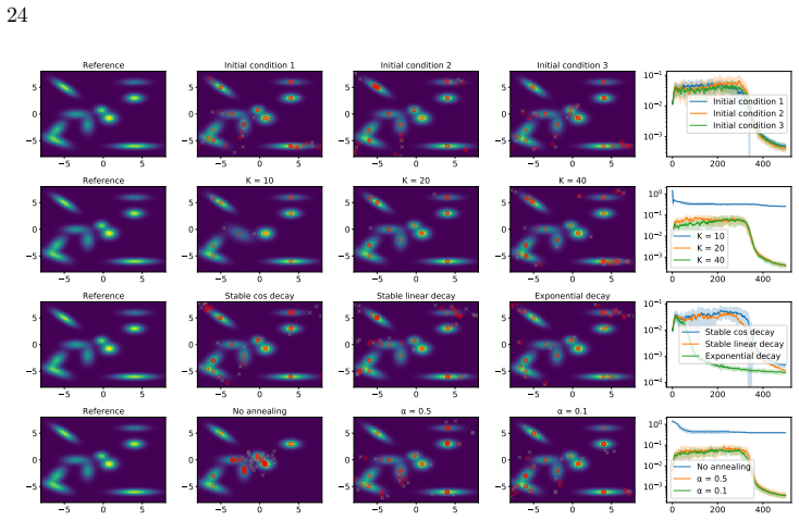
This manuscript is for review purposes only. 24 Fig. 7: Sensitivity study for different choices of initial condition (first row), number of modesK(second row), schedulerη(third row) and annealing strategy (last row) in the 10-dimensional Case A. The fifth panel reports the TV distance between the reference marginal density and the estimated marginal densi...
arXiv 1998
-
[6]
[38]R. E. Kalman,A new approach to linear filtering and prediction problems, J. Basic Eng. Mar, 82 (1960), pp. 35–45. [39]M. Lambert, S. Chewi, F. Bach, S. Bonnabel, and P. Rigollet,Variational inference via wasserstein gradient flows, arXiv preprint arXiv:2205.15902, (2022). [40]B. Li, F. Chen, Z. Huang, L. W ang, and L. Wu,Functional scaling laws in ker...
arXiv 1960
-
[7]
Cao and D
[9]S. Cao and D. Zhengyu Huang,Bayesian calibration for large-scale fluid structure interac- tion problems under embedded/immersed boundary framework, International Journal for Numerical Methods in Engineering, 123 (2022), pp. 1791–1812. [10]J. Carrillo and U. V aes,Wasserstein stability estimates for covariance-preconditioned fokker–planck equations, Non...
2022
-
[559]
[57]M. Welandawe, M. R. Andersen, A. Vehtari, and J. H. Huggins,A framework for improv- ing the reliability of black-box variational inference, Journal of Machine Learning Research, 25 (2024), pp. 1–71, http://jmlr.org/papers/v25/22-0327.html. [58]L. Yan and T. Zhou,An adaptive surrogate modeling based on deep neural networks for large- scale Bayesian inv...
-
[1658]
[24]S. Gershman, M. Hoffman, and D. Blei,Nonparametric variational inference, arXiv preprint arXiv:1206.4665, (2012). [25]J. Goodman and J. Weare,Ensemble samplers with affine invariance, Communications in applied mathematics and computational science, 5 (2010), pp. 65–80. [26]L. Guo, H. Wu, Y. W ang, W. Zhou, and T. Zhou,Ib-uq: Information bottleneck bas...
arXiv 2012
-
[2006]
[6]D. M. Blei, A. Kucukelbir, and J. D. McAuliffe,Variational inference: A review for statisticians, Journal of the American statistical Association, 112 (2017), pp. 859–877. [7]T. Bui-Thanh, O. Ghattas, J. Martin, and G. Stadler,A computational framework for infinite-dimensional Bayesian inverse problems. Part I: The linearized case, with appli- cation t...
2017
-
[2008]
[48]M. Opper and C. Archambeau,The variational Gaussian approximation revisited, Neural computation, 21 (2009), pp. 786–792. [49]J. Paisley, D. Blei, and M. Jordan,Variational Bayesian inference with stochastic search, arXiv preprint arXiv:1206.6430, (2012). [50]X. Pennec, P. Fillard, and N. Ayache,A riemannian framework for tensor computing, Internationa...
arXiv 2009
-
[2275]
[11]J. A. Carrillo, Y. Chen, D. Z. Huang, J. Huang, and D. Wei,Fisher-rao gradient flow: geodesic convexity and functional inequalities, arXiv preprint arXiv:2407.15693, (2024). [12]N. K. Chada, A. M. Stuart, and X. T. Tong,Tikhonov regularization within ensemble Kalman inversion, SIAM Journal on Numerical Analysis, 58 (2020), pp. 1263–1294. This manuscri...
arXiv 2024
Reviewed August 3, 2026 · model on record in the stance chip above.
Discussion (0). Continue with ORCID to comment.