REVIEW 5 major objections 5 minor 2 references
A strictly geostrophic product of sea-surface velocities from the SWOT fast-sampling phase
T0 review · 5 major / 5 minor · reviewed 2026-08-03 · deepseek-v4-flash
Pith's one-line read A frequency-domain decomposition of SWOT's daily repeat orbit isolates a strictly geostrophic sea-surface height field, resolving the ambiguity of spatial filtering and matching drifters at least as well as the default product.
desk verdict A useful global extension of an existing DMD decomposition to all SWOT fast-sampling passes, but the 'strictly geostrophic' claim is stronger than the evidence supports because the key validation conflates spatial smoothing with temporal filtering. read the letter →
The pith
A machine-rendered reading of the paper's core claim, the machinery that carries it, and where it could break.
The reading
What carries the argument
mrCOSTS — multi-resolution COherent Spatio-Temporal scale Separation, a recursive dynamic-mode-decomposition variant that assigns each spatial pattern a temporal frequency without requiring periodic boundaries. It is applied over four levels with window lengths of 9, 10, 30 and 60 days, and the geostrophic component is the sum of modes with frequency below 0.1 cycles per day. The companion mechanism is internal-tide preprocessing: the default empirical tide product is added back, then internal-tide sea-surface signals from an ocean forecast model are subtracted, so that remaining variability is mostly free of both coherent and incoherent internal tides before the frequency split.
What would settle it
Run the same mrCOSTS pipeline on synthetic SWOT-like observations generated from a model with known geostrophic and ageostrophic fields and compare the extracted sub-0.1-cycles-per-day height to the known truth; alternatively, check the released product for residual variance at diurnal and semidiurnal frequencies. If residual tidal variance is significant or the reconstructed geostrophic field deviates from truth beyond sampling error, the strict-geostrophy claim fails.
Extended reading notes
Core claim
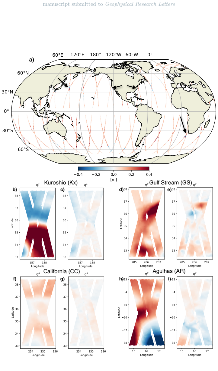
The central claim is that geostrophy is a low-frequency balance, and that temporal information from SWOT's fast-sampling orbit can be used to enforce it, rather than relying on spatial scale alone. The geostrophic sea-surface height field, ηg, is constructed by summing mrCOSTS modes with frequencies below 0.1 cycles per day, after a two-step internal-tide removal. The resulting fields evolve on scales slower than about ten days and larger than about one hundred kilometres. The paper shows that vorticity and strain normalized by the inertial frequency are mostly smaller than order one in the mrCOSTS product, whereas applying geostrophy directly to the de-tided SWOT field gives fatter tails ab
Load-bearing premise
The decomposition rests on the assumption that the ocean forecast model's internal-tide correction removes essentially all internal-tide sea-surface height, so that any residual tidal energy is not mistaken for low-frequency geostrophic motion.
Editorial extensions
If this is right
- Spatial filtering alone is insufficient: applying geostrophic balance directly to the de-tided SWOT field produces vorticity and strain values above the small-Rossby-number threshold, so the standard approach is shown to contain ageostrophic contamination.
- The released global geostrophic fields enable geostrophic kinetic-energy cascade estimates and quasi-geostrophic omega-equation vertical velocity reconstructions without the high-frequency, high-wavenumber noise present in the residual ageostrophic component.
- The frequency cutoff at 0.1 cycles per day makes the temporal definition of geostrophy explicit: only signals with periods longer than ten days and wavelengths above roughly 100 km are treated as balanced.
- The fast-sampling orbit's daily repeats are sufficient for the method, while the science orbit's sparse repeats — about 50 per pass — are not yet enough, so the product's scope is tied to the duration and repeat rate of the calibration/validation phase.
Reading between the lines
- A sensitivity test varying the 0.1 cycles-per-day cutoff and the SVD ranks would show how much of the improvement in vorticity and strain statistics is a consequence of the filter choice rather than an intrinsic property of the ocean signal.
- If the frequency-based separation is as clean as claimed, the same machinery could be applied to other altimetry data with irregular temporal sampling once enough repeat observations accumulate, rather than waiting for a dedicated fast-sampling orbit.
- The Mediterranean drifter comparison is the only direct velocity validation; a natural next test is to validate the global product against drifters or current meters in the energetic Agulhas and Gulf Stream regions examined in the paper, where the vorticity-strain diagnostics are strongest.
- The paper attributes the missing cyclonic skewness in the vorticity distribution to the short three-month record; as SWOT data accumulate, one can test whether longer records restore the expected skewness or whether the frequency filter itself suppresses it.
Signed reviews
Editorial analysis
A structured set of objections, weighed in public.
Referee Report
Summary. This paper applies the multi-resolution coherent spatio-temporal scale separation (mrCOSTS) dynamic mode decomposition to the global SWOT fast-sampling phase (March 29–July 11, 2023) Level-3 sea-surface height anomalies. The authors replace the default HRET internal-tide correction with a HYCOM forecast correction, then define a 'strictly geostrophic' component ηg as the sum of mrCOSTS modes with frequency <0.1 cpd (periods >10 days). They process every SWOT pass, promise public distribution of the global product, and evaluate it via frequency–wavenumber spectra at four cross-over regions, joint PDFs of vorticity and strain, and a comparison to SVP drifters in the western Mediterranean Sea. The main claims are that mrCOSTS overcomes spectral leakage due to temporal aliasing, that ηg has Rossby numbers mostly below unity, and that its velocity estimates agree with drifters at least as well as the default L3HRET product while reducing speed bias.
Significance. If fully supported, the paper would provide a practical, global method for exploiting the temporal dimension of the 1-day-repeat SWOT orbit to separate balanced motions from internal tides and ageostrophic eddies, avoiding the arbitrary spatial-filter choices common in SWOT analyses. The pipeline is clearly documented, the code is available, the HYCOM-based IT correction is state-of-the-art, and the authors are transparent about residual limitations (e.g., missing cyclonic skewness, short Cal/Val record, limited drifter sample). A publicly distributed global geostrophic product would be a valuable community resource. However, the validation as presented does not isolate the DMD temporal filter from the Gaussian spatial pre-filter, and the drifter comparison lacks a quantitative skill metric. Thus the central claims are defensible but not yet fully supported.
major comments (5)
- [§3.2, Fig. 3] The head-to-head comparison of ζg/|f| and |αg|/|f| between mrCOSTS ηg and L3HYCOM confounds the temporal DMD filtering (Steps 5–6) with the Gaussian spatial filter of Step 3, which is applied only to mrCOSTS. Vorticity and strain amplify small-scale gradients, so the reduced tails in the mrCOSTS PDFs could be produced entirely by the ~6 km spatial smoothing. The text states the spatial smoothing is 'not used to extract the geostrophic component,' but no control product is shown. Please add a comparison of L3HYCOM after the same Gaussian filter, and ideally after a simple temporal low-pass filter, to isolate the DMD contribution. Without such a control, the central claim that mrCOSTS 'overcomes spectral leakage' is not established.
- [§2.1, Step 6; §3.1, Fig. 2] The sharp spectral cutoff at 10 days in the ω–k spectra of ηg is partly circular: ηg is defined as the sum of modes with frequency <0.1 cpd, so the observed cutoff restates the construction. The statement in §3.1 that 'there is a clear cutoff of power at time scales shorter than 10 days' acknowledges this, but it does not validate geostrophic character. Independent evidence must come from the drifter comparison or from a quantitative skill metric; the Rossby-number contrast is confounded per the preceding comment. Please provide a non-circular diagnostic, for example the fraction of spectral energy of ηg at periods just below and above 10 days, or a comparison to a model balanced component.
- [§3.3, Fig. 4] The drifter validation is qualitative and geographically narrow. The paper itself notes that L3HRET is 'slightly better aligned' (smaller angular spread) than mrCOSTS, while mrCOSTS reduces speed bias, but the claim 'at least as good as if not better' is not backed by a statistical measure. Please provide quantitative error statistics (e.g., complex correlation, median and interquartile range of the ratio, circular standard deviation) with uncertainty estimates. Consider extending the analysis to more than one Mediterranean pass or to other regions with available in situ data, or explicitly frame the results as a single-region case study.
- [§2.1, Step 1] The entire product rests on the assumption that the HYCOM forecast internal-tide correction removes essentially all incoherent IT energy after 'add back HRET, subtract HYCOM.' Any residual IT variance would be classified as geostrophic by the <0.1 cpd cutoff. The paper provides no independent check of residual tidal variance in ηg (e.g., spectral energy at M2/K1 frequencies or comparison to tide-gauge/current-meter data). If Yadidya et al. (2025) contains such validation, cite the specific evidence; otherwise add a diagnostic to the manuscript.
- [§2.1, Step 5] The mrCOSTS hyperparameters (window lengths [9,10,30,60] days, SVD ranks [4,4,10,12]) and the 0.1 cpd geostrophic-frequency cutoff are set by hand with no sensitivity analysis. DMD/mrCOSTS modes can depend nontrivially on windowing and rank truncation. A sensitivity test (e.g., varying the cutoff between 0.08 and 0.12 cpd, adjusting window/rank choices) is needed to show that the main conclusions—PDFs, spectra, drifter agreement—are robust. This is especially important because the 'strictly geostrophic' claim is the paper's central contribution.
minor comments (5)
- [Author list] The author affiliation contains repeated/odd characters in the Chinese transliteration ('内 内 内田 田 田貴 貴 貴也 也 也'), likely a LaTeX artifact; please fix.
- [§2.1, Step 3] The Gaussian filter is described as having standard deviation 'of three grid points (~6km).' Please specify the nominal grid spacing and whether the filter is isotropic in both along-track and cross-track directions.
- [§3.1] The text states that the geostrophic spectra 'peaks at scales larger than 100 km and slower than 20 days,' which is inconsistent with the 10-day cutoff in Fig. 2 and Step 6. Should read '10 days' unless a different frequency range is intended.
- [§3.2, Fig. 3] The caption of Fig. 3 uses 'mrCOASTS' in one panel label; should be 'mrCOSTS' for consistency. Also, the sentence in §3.2 'the joint PDFs are documenting that geostrophic balance was applied to SSHa signals in L3HYCOM that were in fact not in balance' could be rephrased more concisely.
- [§3.3, Fig. 4] The polar-histogram labels in Fig. 4 use 'Drifter / L3' and 'Drifter / mrCOSTS' but the text refers to the L3HRET product; please harmonize notation. The rotary-spectra caption would benefit from explicitly describing which curves correspond to the 25-hr and 48-hr filters.
Circularity Check
The ω-k 'cutoff at 10 days' restates Step 6's frequency selection; drifter and Rossby-number checks are external and keep the central product from collapsing.
-
self definitional
[Section 3.1 (Fig. 2) and Section 2.1, Step 6]
"Notably, there is a clear cutoff of power at time scales shorter than 10 days as expected from the mrCOSTS frequencies (Step 6 in Section 2.1; Fig. 2a,c,e,g)."
ηg is constructed, in Step 6, by summing only mrCOSTS modes with frequencies smaller than 0.1 cpd, i.e., periods longer than 10 days. The reported 'clear cutoff of power at time scales shorter than 10 days' is therefore the selection rule restated in spectral form, not an independent property of the extracted component. The associated bullet in the Discussion—'ηg evolves on time scales slower than O(10 days)'—uses the same by-construction property as if it were a validation of the decomposition. The ageostrophic field ηa is by definition the complement, so its faster-than-10-day tail is equally constructed rather than discovered.
full rationale
The paper's central product is a data-processing pipeline (HYCOM detiding, 6-km Gaussian prefilter, mrCOSTS DMD, sub-0.1-cpd mode sum) and the main external evidence—the SVP drifter polar histograms and vorticity-strain PDFs—does not reduce to the construction. The one clearly circular element is the frequency-domain result: the Fig. 2 cutoff at 10 days is inserted by Step 6, and Section 4's claim that mrCOSTS 'overcomes ... spectral leakage' and produces modes 'at frequencies distinctly lower than the Nyquist frequency' is likewise guaranteed in part by the 0.1-cpd selection rule. The paper is transparent about this ('as expected from the mrCOSTS frequencies'), which lowers the severity. The comparison against L3HYCOM is also confounded by the Gaussian prefilter, since L3HYCOM is not passed through the same spatial smoothing; that is a validation confound rather than a circular reduction. The HYCOM IT-correction premise is supported by prior published work (Yadidya et al., 2024, 2025) with overlapping authors, but it is an external dataset/study rather than an ansatz smuggled in by citation, so it does not by itself make the argument circular. Weighing the by-construction spectral diagnostics against the independent drifter and PDF checks yields a partial-circularity score of 4.
Assumptions & free parameters
free parameters (5)
- mrCOSTS window lengths =
[9, 10, 30, 60] days
- SVD ranks =
[4, 4, 10, 12]
- Geostrophic frequency cutoff =
0.1 cpd (10-day period)
- Gaussian spatial filter standard deviation =
3 grid points (~6 km)
- Drifter low-pass filter cutoff =
48 hours
assumptions (5)
- domain assumption Geostrophic balance is valid for motions with time scales longer than the inertial period and spatial scales larger than the deformation radius.
- domain assumption The HYCOM forecast removes both coherent and incoherent internal tides from SWOT SSHa.
- domain assumption mrCOSTS/DMD correctly separates spatiotemporal modes from one-day-sampled SWOT data without spectral leakage.
- domain assumption Bilinear spatial interpolation of missing data and zero-filling of land/islands do not bias the extracted modes.
- domain assumption Drifter velocities, after Ekman removal and 48-hour low-pass filtering, are a suitable reference for the geostrophic product.
Cite this review
Pith. "Pith review of A strictly geostrophic product of sea-surface velocities from the SWOT fast-sampling phase." pith.science (2026). https://pith.science/paper/3J3BJ6R6
@misc{pith2026260118182,
  author       = {Pith},
  title        = {Pith review of: A strictly geostrophic product of sea-surface velocities from the SWOT fast-sampling phase},
  year         = {2026},
  howpublished = {\url{https://pith.science/paper/3J3BJ6R6}},
  note         = {Machine review of arXiv:2601.18182}
}
read the original abstract
While geostrophy remains the simplest and most practical balance to extract velocity information from sea-surface height anomaly (SSHa), confusions remain within the oceanographic community to what extent this balance can be applied to altimetric observations with the launch of the Surface Water and Ocean Topography (SWOT) satellite. Given the limited temporal resolution of SWOT, many studies have resorted to claiming that the spatially filtered SSHa fields correspond to the geostrophic component. This introduces the ambiguity of which spatial scale to choose. Here, we build upon the recent developments in internal tide (IT) corrections (Yadidya et al., 2025) and apply a dynamic mode decomposition (DMD)-based method introduced by Lapo et al. (2025) to robustly extract the geostrophic component associated with sub-inertial frequencies from the SWOT one-day-repeat orbit; we distribute the global dataset as a public good. We provide the joint probability density function (PDF) of vorticity and strain, and spectra of SSHa at a few cross-over regions.
Figures


Figures from the paper (1 more)

Reference graph
Works this paper leans on
-
[1]
P., Squire, D., Bourbeau, J., Nicholas, T., Bourbeau, J., Joseph, G.,
Abernathey, R. P., Squire, D., Bourbeau, J., Nicholas, T., Bourbeau, J., Joseph, G., ... others (2023).xhistogram: Fast, flexible, label-aware histograms for numpy and xarray [Software].Zenodo. Retrieved fromhttps:// xhistogram.readthedocs.io/en/latest/doi: 10.5281/zenodo.7095156 AVISO/DUACS. (2025).SWOT Level-3 KaRIn Low Rate SSH Expert (v2.0.1) [Dataset...
arXiv 2023
-
[530]
Retrieved fromhttps:// pydmd.github.io/PyDMD/doi: 10.21105/joss.00530 Demol, M., Berta, M., Gomez Navarro, L., Izard, L., Ardhuin, F., Bellacicco, M., ... Verger-Miralles, E. (2023).A drifter dataset for the western Mediterranean Sea collected during the SWOT mission calibration and validation phase [Dataset]. Seanoe. doi: 10.17882/100828 Dias, S., Surasi...
Reviewed August 3, 2026 · model on record in the stance chip above.
Discussion (0). Continue with ORCID to comment.