Optimized k-means color quantization of digital images in machine-based and human perception-based colorspaces
Pith reviewed 2026-05-25 07:17 UTC · model grok-4.3
The pith
k-means color quantization yields highest visual fidelity in RGB for about half of images, with CIE-XYZ better at higher k and CIE-LUV at lower k in some cases.
A machine-rendered reading of the paper's core claim, the machinery that carries it, and where it could break.
Core claim
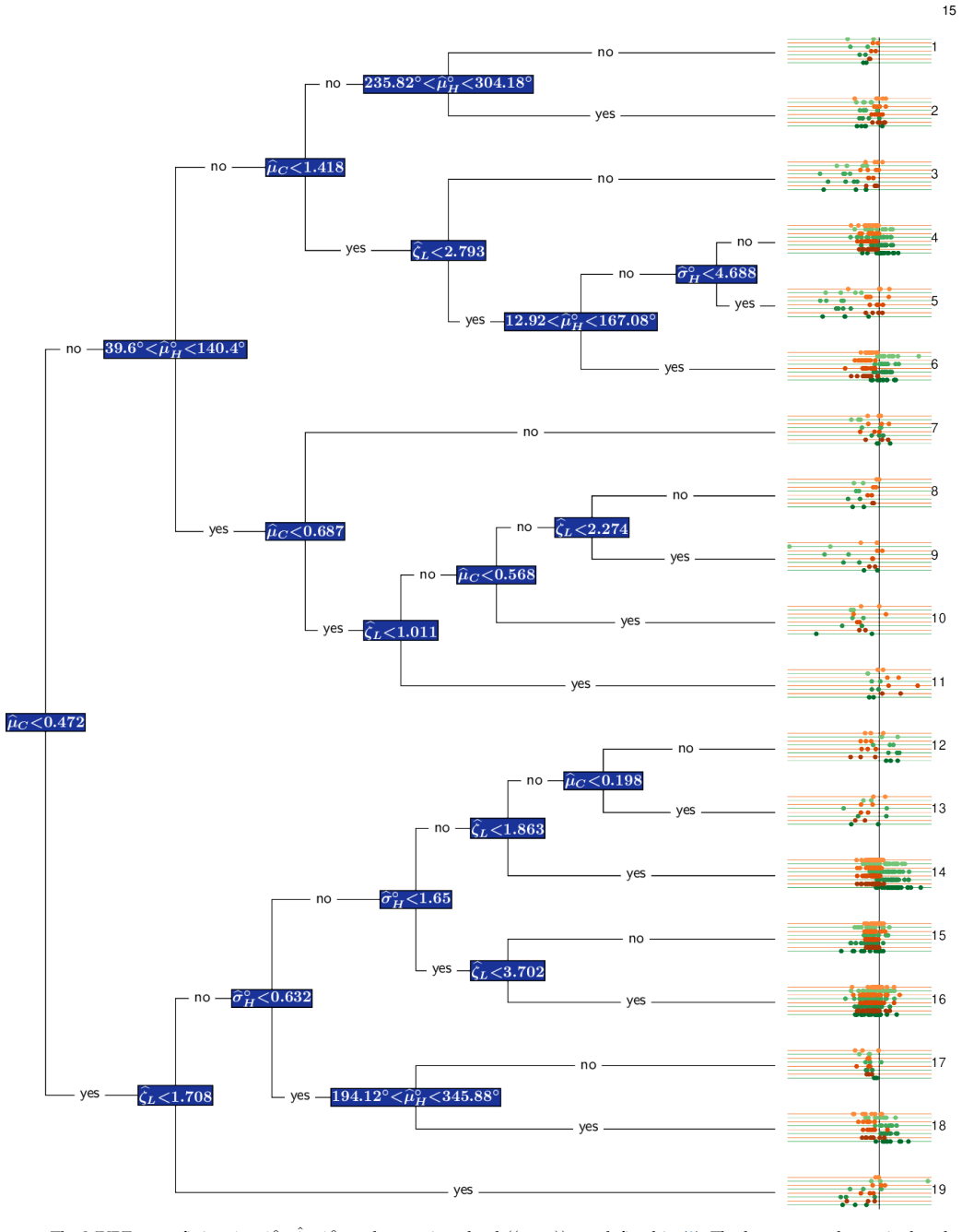
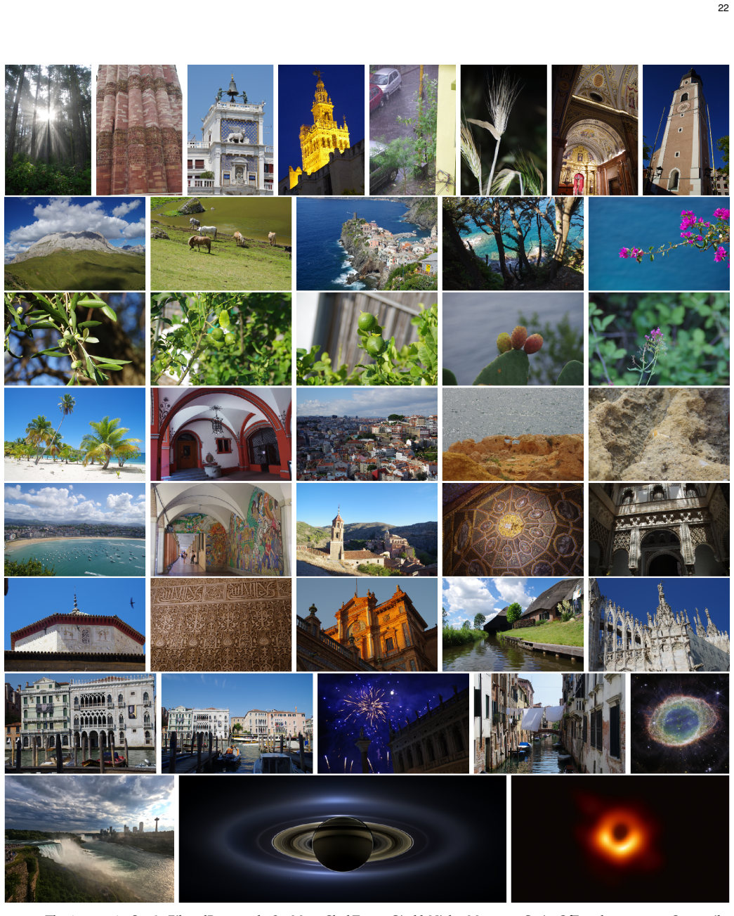
k-means color quantization produces the highest Visual Information Fidelity scores in the RGB colorspace for about half of the 148 tested images across quantization levels, while the CIE-XYZ colorspace yields better results in the remaining cases, particularly at higher k, and the CIE-LUV colorspace performs best in some instances at lower k. Distributions of hue, chromaticity, and luminance in the original images provide a way to characterize when each colorspace is preferable.
What carries the argument
Performance comparison of k-means clustering for color quantization across RGB, CIE-XYZ, and CIE-LUV/CIE-HCL spaces, scored by Visual Information Fidelity on 148 images at multiple k levels, plus analysis of hue, chromaticity, and luminance distributions.
If this is right
- At higher quantization levels, using CIE-XYZ instead of RGB can improve the fidelity of the reduced-color image.
- At lower k, testing CIE-LUV may give better results for images with particular hue or luminance properties.
- No single colorspace is optimal for all images, so selection can depend on image content statistics.
- Further breakdown by hue, chromaticity, and luminance distributions can guide practical choices of colorspace for quantization.
Where Pith is reading between the lines
- An adaptive algorithm could select the colorspace automatically based on quick statistics of an image's luminance and hue distribution.
- The approach might extend to other clustering-based image processing tasks where color representation affects output quality.
- Validation against actual human perception studies would clarify whether the VIF differences are noticeable to viewers.
- These patterns could inform color quantization steps in image compression or web image optimization pipelines.
Load-bearing premise
The Visual Information Fidelity metric provides a reliable numerical proxy for human-perceived visual quality when comparing quantized images produced in different colorspaces.
What would settle it
Human viewer preference rankings on a sample of the quantized image pairs that contradict the VIF-based ordering of which colorspace performed best.
Figures


read the original abstract
Color quantization represents an image using a fraction of its original number of colors while only minimally losing its visual quality. The $k$-means algorithm is commonly used in this context, but has mostly been applied in the machine-based RGB colorspace composed of the three primary colors. However, some recent studies have indicated its improved performance in human perception-based colorspaces. We investigated the performance of $k$-means color quantization at four quantization levels in the RGB, CIE-XYZ, and CIE-LUV/CIE-HCL colorspaces, on 148 varied digital images spanning a wide range of scenes, subjects and settings. The Visual Information Fidelity (VIF) measure numerically assessed the quality of the quantized images, and showed that in about half of the cases, $k$-means color quantization is best in the RGB space, while at other times, and especially for higher quantization levels ($k$), the CIE-XYZ colorspace is where it usually does better. There are also some cases, especially at lower $k$, where the best performance is obtained in the CIE-LUV colorspace. Further analysis of the performances in terms of the distributions of the hue, chromaticity and luminance in an image presents a nuanced perspective and characterization of the images for which each colorspace is better for $k$-means color quantization.
Editorial analysis
A structured set of objections, weighed in public.
Referee Report
Summary. The manuscript empirically compares k-means color quantization performance in RGB, CIE-XYZ, and CIE-LUV (and CIE-HCL) colorspaces across 148 varied images at four quantization levels. Quality is assessed via the Visual Information Fidelity (VIF) metric, leading to the claim that RGB performs best in roughly half the cases, CIE-XYZ is often superior at higher k, and CIE-LUV at lower k; additional analysis examines image hue, chromaticity, and luminance distributions to characterize when each space is preferable.
Significance. If the VIF-based rankings are reliable across colorspaces, the work supplies practical empirical guidance on colorspace choice for k-means quantization, which could inform compression, display, and machine-vision pipelines. The study is strengthened by its use of a sizable, diverse image corpus rather than synthetic or narrow test sets.
major comments (1)
- [Abstract] Abstract: The central empirical claim (RGB best in ~half the cases, XYZ at higher k, LUV at lower k) rests solely on VIF scores. VIF was formulated for luminance-channel distortions; the manuscript provides no validation (e.g., cross-check against CIEDE2000 on the same quantized images or subjective ratings) that VIF rankings remain consistent when the same results are produced in XYZ versus LUV and then converted to a common space for scoring. Systematic bias is possible because quantization error distributions affect chromatic channels differently across spaces.
minor comments (2)
- [Abstract] Abstract: The four specific quantization levels (k values) are not stated.
- [Abstract] Abstract: No information is given on statistical testing, exact image-selection criteria, or potential confounds such as content category balance.
Simulated Author's Rebuttal
We thank the referee for the careful reading and for highlighting a methodological point regarding the VIF metric. We address the concern directly below and indicate the revisions we are prepared to make.
read point-by-point responses
-
Referee: [Abstract] Abstract: The central empirical claim (RGB best in ~half the cases, XYZ at higher k, LUV at lower k) rests solely on VIF scores. VIF was formulated for luminance-channel distortions; the manuscript provides no validation (e.g., cross-check against CIEDE2000 on the same quantized images or subjective ratings) that VIF rankings remain consistent when the same results are produced in XYZ versus LUV and then converted to a common space for scoring. Systematic bias is possible because quantization error distributions affect chromatic channels differently across spaces.
Authors: We agree that VIF was originally derived for luminance distortions and that its behavior when applied to full-color images quantized in different spaces merits explicit checking. In the manuscript we convert all quantized results to sRGB before computing VIF, which places the final images in a common coordinate system; however, we did not report a secondary metric such as CIEDE2000 or any subjective validation. We will therefore add a supplementary section that recomputes the per-image, per-k rankings using CIEDE2000 on the same set of quantized images and reports the agreement rate between VIF and CIEDE2000 orderings. This addition will quantify any systematic discrepancy introduced by the choice of VIF. We view the requested check as a useful strengthening of the evidence rather than a refutation of the current conclusions. revision: partial
Circularity Check
No circularity: purely empirical comparison of k-means in colorspaces via VIF
full rationale
The paper reports direct experimental results from running k-means quantization on 148 images in RGB, CIE-XYZ, and CIE-LUV/HCL spaces, then ranking the outputs by VIF scores. No equations, fitted parameters, predictions, or self-citations are used to derive the central claims (RGB best in ~half the cases, XYZ at higher k, LUV at lower k). The VIF application is a fixed external metric, not redefined or fitted within the paper. No load-bearing steps reduce to inputs by construction.
Axiom & Free-Parameter Ledger
axioms (1)
- domain assumption VIF is an appropriate metric for assessing quantized image quality in different color spaces
Reference graph
Works this paper leans on
-
[1]
J. D. Murray and W. vanRyper,Encyclopedia of Graphics File Formats, 2nd ed. O’Reilly, 1996
work page 1996
-
[2]
The use and manipulation of digital image files in light microscopy,
E. H. Hinchcliffe, “The use and manipulation of digital image files in light microscopy,”Methods in cell biology, pp. 271–289, 2003
work page 2003
-
[3]
T. Acharya, “Integrated color interpolation and color space conversion algorithm from 8-bit Bayer pattern RGB color space to 24-bit CIE XYZ color space,” Apr. 2 2002, uS Patent 6,366,694
work page 2002
-
[4]
Colour image quantization for high resolution graphics display,
N. Goldberg, “Colour image quantization for high resolution graphics display,”Image and vision computing, vol. 9, no. 5, pp. 303–312, 1991
work page 1991
-
[5]
Color spaces for computer graphics,
G. H. Joblove and D. Greenberg, “Color spaces for computer graphics,” inACM siggraph computer graphics, vol. 12, no. 3. ACM, 1978, pp. 20–25
work page 1978
-
[6]
A. Ford and A. Roberts, “Colour space conversions,” url = https://poynton.ca/PDFs/coloureq.pdf, pp. 1–31, 1998
work page 1998
-
[7]
C.-K. Yang and W.-H. Tsai, “Color image compression using quantization, thresholding, and edge detection techniques all based on the moment-preserving principle,”Pattern Recognition Letters, vol. 19, no. 2, pp. 205–215, 1998
work page 1998
-
[8]
Improving the performance of k-means for color quantization,
M. E. Celebi, “Improving the performance of k-means for color quantization,”Image and Vision Computing, vol. 29, no. 4, pp. 260–271, 2011
work page 2011
-
[9]
Bootstrapping for significance of compact clusters in multidimensional datasets,
R. Maitra, V . Melnykov, and S. N. Lahiri, “Bootstrapping for significance of compact clusters in multidimensional datasets,”Journal of the American Statistical Association, vol. 107, no. 497, pp. 378–392, 2012
work page 2012
-
[10]
Forty years of color quantization: a modern, algorithmic survey,
M. E. Celebi, “Forty years of color quantization: a modern, algorithmic survey,”Artificial Intelligence Review, vol. 56, p. 13953–14034, 2023
work page 2023
-
[11]
Color image quantization by minimizing the maximum intercluster distance,
Z. Xiang, “Color image quantization by minimizing the maximum intercluster distance,”ACM Transactions on Graphics (TOG), vol. 16, no. 3, pp. 260–276, 1997
work page 1997
-
[12]
An effective color quantization method based on the competitive learning paradigm,
M. Celebi, “An effective color quantization method based on the competitive learning paradigm,” inProceedings of the 2009 International Conference on Image Processing, Computer Vision, and Pattern Recognition, vol. 2, 2009, p. 876–880
work page 2009
-
[13]
Neural gas clustering for color reduction,
M. Celebi and G. Schaefer, “Neural gas clustering for color reduction,” inProceedings of the 2010 International Conference on Image Processing, Computer Vision, and Pattern Recognition, vol. 1, 2010, p. 429–432
work page 2010
-
[14]
G. Schaefer, H. Zhou, M. E. Celebi, and A. E. Hassanien, “Rough colour quantisation,”International Journal of Hybrid Intelligent Systems, vol. 8, p. 25–30, 2011
work page 2011
-
[15]
Fuzzy algorithm for color quantization of images,
D. Ozdemir and L. Akarun, “Fuzzy algorithm for color quantization of images,”Pattern Recognition, vol. 35, no. 8, p. 1785–1791, 2002
work page 2002
-
[16]
Fuzzy clustering for colour reduction in images,
G. Schaefer and H. Zhou, “Fuzzy clustering for colour reduction in images,”Telecommunication Systems, vol. 40, no. 1–2, p. 17–25, 2009
work page 2009
-
[17]
An adjustable algorithm for color quantization,
Z. Bing, S. Junyi, and P . Qinke, “An adjustable algorithm for color quantization,”Pattern Recognition Letters, vol. 25, no. 16, p. 1787–1797, 2004
work page 2004
-
[18]
Kohonen neural networks for optimal colour quantization,
A. Dekker, “Kohonen neural networks for optimal colour quantization,”Network: Computation in Neural Systems, vol. 5, no. 3, p. 351–367, 1994
work page 1994
-
[19]
N. Papamarkos, A. Atsalakis, and C. Strouthopoulos, “Adaptive color reduction,”IEEE Transactions on Systems, Man, and Cybernetics, vol. 32, no. 1, p. 44–56, 2002
work page 2002
-
[20]
New adaptive color quantization method based on self-organizing maps,
C.-H. Chang, P . Xu, R. Xiao, and T. Srikanthan, “New adaptive color quantization method based on self-organizing maps,”IEEE Transactions on Neural Networks, vol. 16, no. 1, p. 237–249, 2005
work page 2005
-
[21]
Color quantization using an accelerated Janceyk-means clustering algorithm,
H. Bounds, M. E. Celebi, and J. Maxwell, “Color quantization using an accelerated Janceyk-means clustering algorithm,”Journal of Electronic Imaging, vol. 33, no. 5, p. 053052, 2024. [Online]. Available: https://doi.org/10.1117/1.JEI.33.5.053052
-
[22]
Algorithm AS 136: Ak-means clustering algorithm,
J. A. Hartigan and M. A. Wong, “Algorithm AS 136: Ak-means clustering algorithm,”Journal of the Royal Statistical Society. Series C (Applied Statistics), vol. 28, no. 1, pp. 100–108, 1979
work page 1979
-
[23]
Least squares quantization in PCM,
S. Lloyd, “Least squares quantization in PCM,”IEEE Transactions on Information Theory, vol. 28, no. 2, p. 129–136, 1982
work page 1982
-
[24]
Localk-means algorithm for colour image quantization,
O. Verevka and J. Buchanan, “Localk-means algorithm for colour image quantization,” inProceedings of the Graphics/Vision Interface Conference, 1995, p. 128–135
work page 1995
-
[25]
Comparison of clustering algorithms applied to color image quantization,
P . Scheunders, “Comparison of clustering algorithms applied to color image quantization,”Pattern Recognition Letters, vol. 18, no. 11–13, p. 1379–1384, 1997
work page 1997
-
[26]
CQ100: a high-quality image dataset for color quantization research,
M. E. Celebi and M.-L. P ´erez-Delgado, “CQ100: a high-quality image dataset for color quantization research,”Journal of Electronic Imaging, vol. 32, no. 3, p. 033019, 2023. [Online]. Available: https://doi.org/10.1117/1.JEI.32.3.033019 24
-
[27]
A comparative study of color quantization methods using various image quality assessment indices,
L. P ´erez-Delgado, M and M. E. Celebi, “A comparative study of color quantization methods using various image quality assessment indices,” Multimedia Systems, vol. 30, no. 40, 2024
work page 2024
-
[28]
An information fidelity criterion for image quality assessment using natural scene statistics,
H. Sheikh, A. Bovik, and G. de Veciana, “An information fidelity criterion for image quality assessment using natural scene statistics,”IEEE Transactions on Image Processing, vol. 14, no. 12, pp. 2117–2128, 2005
work page 2005
-
[29]
Image information and visual quality,
H. Sheikh and A. Bovik, “Image information and visual quality,”IEEE Transactions on Image Processing, vol. 15, no. 2, pp. 430–444, 2006
work page 2006
- [30]
-
[31]
J. Schanda,CIE Colorimetry. John Wiley & Sons, Ltd, 2007, ch. 3, pp. 25–78. [Online]. Available: https://onlinelibrary.wiley.com/doi/abs/ 10.1002/9780470175637.ch3
-
[32]
Accurate color reproduction for computer graphics applications,
B. J. Lindbloom, “Accurate color reproduction for computer graphics applications,”ACM SIGGRAPH Computer Graphics, vol. 23, no. 3, pp. 117–126, 1989
work page 1989
-
[33]
J. Y. Hardeberg,Acquisition and Reproduction of Color Images: Colorimetric and Multispectral Approaches. Universal-Publishers.com, 2001
work page 2001
-
[34]
Calibrated color measurements of agricultural foods using image analysis,
F. Mendoza, P . Dejmek, and J. M. Aguilera, “Calibrated color measurements of agricultural foods using image analysis,”Postharvest Biology and Technology, vol. 41, no. 3, pp. 285–295, 2006
work page 2006
-
[35]
The CIE XYZ and xyY color spaces,
D. A. Kerr, “The CIE XYZ and xyY color spaces,” url = https://graphics.stanford.edu/courses/cs148-10-summer/docs/2010–kerr–cie xyz.pdf , 2010
work page 2010
-
[36]
Chromatic characterization of anthocyanins from red grapes—i. ph effect,
F. J. Heredia, E. M. Francia-Aricha, J. C. Rivas-Gonzalo, I. M. Vicario, and C. Santos-Buelga, “Chromatic characterization of anthocyanins from red grapes—i. ph effect,”Food Chemistry, vol. 63, no. 4, pp. 491–498, 1998
work page 1998
-
[37]
Fast colour space transformations using minimax approximations,
M. E. Celebi, H. A. Kingravi, and F. Celiker, “Fast colour space transformations using minimax approximations,”Image Processing, IET, vol. 4, no. 2, pp. 70–80, 2010
work page 2010
-
[38]
21 - the CIE system of colorimetry,
C. Poynton, “21 - the CIE system of colorimetry,” inDigital Video and HDTV, ser. The Morgan Kaufmann Series in Computer Graphics, C. Poynton, Ed. San Francisco: Morgan Kaufmann, 2003, pp. 211–231. [Online]. Available: https: //www.sciencedirect.com/science/article/pii/B9781558607927500872
work page 2003
-
[39]
Escaping rgbland: Selecting colors for statistical graphics,
A. Zeileis, K. Hornik, and P . Murrell, “Escaping rgbland: Selecting colors for statistical graphics,”Computational Statistics & Data Analysis, vol. 53, no. 9, pp. 3259–3270, 2009. [Online]. Available: https://www.sciencedirect.com/science/article/pii/S0167947308005549
work page 2009
-
[40]
Historical development of cie recommended color difference equations,
A. R. Robertson, “Historical development of cie recommended color difference equations,”Color Research & Application, vol. 15, no. 3, pp. 167–170, 1990. [Online]. Available: https://onlinelibrary.wiley.com/doi/abs/10.1002/col.5080150308
-
[41]
Model-based halftoning of color images,
T. Pappas, “Model-based halftoning of color images,”IEEE Transactions on Image Processing, vol. 6, no. 7, pp. 1014–1024, 1997
work page 1997
-
[42]
Y. Sirisathitkul, S. Auwatanamongkol, and B. Uyyanonvara, “Color image quantization using distances between adjacent colors along the color axis with highest color variance,”Pattern Recognition Letters, vol. 25, no. 9, pp. 1025–1043, 2004
work page 2004
-
[43]
Computational improvements to the kernelk-means clustering algorithm,
J. D. Berlinski and R. Maitra, “Computational improvements to the kernelk-means clustering algorithm,”Statistical Analysis and Data Mining: An ASA Data Science Journal, vol. 18, no. 4, p. e70032, 2025. [Online]. Available: https://onlinelibrary.wiley.com/doi/abs/10.1002/sam.70032
-
[44]
Color image quantization for frame buffer display,
P . Heckbert, “Color image quantization for frame buffer display,”SIGGRAPH Comput. Graph., vol. 16, no. 3, p. 297–307, Jul. 1982. [Online]. Available: https://doi.org/10.1145/965145.801294
-
[45]
A fast pixel mapping algorithm using principal component analysis,
K.-F. Hwang and C.-C. Chang, “A fast pixel mapping algorithm using principal component analysis,”Pattern recognition letters, vol. 23, no. 14, pp. 1747–1753, 2002
work page 2002
-
[46]
Relative clustering validity criteria: A comparative overview,
L. Vendramin, R. J. G. B. Campello, and E. R. Hruschka, “Relative clustering validity criteria: A comparative overview,” Statistical Analysis and Data Mining: The ASA Data Science Journal, vol. 3, no. 4, pp. 209–235, 2010. [Online]. Available: https://onlinelibrary.wiley.com/doi/abs/10.1002/sam.10080
-
[47]
Some methods for classification and analysis of multivariate observations,
J. MacQueen, “Some methods for classification and analysis of multivariate observations,”Proceedings of the Fifth Berkeley Symposium, vol. 1, pp. 281–297, 1967
work page 1967
-
[48]
Hartigan’s method: k-means clustering without Voronoi,
M. Telgarsky and A. Vattani, “Hartigan’s method: k-means clustering without Voronoi,” inProceedings of the Thirteenth International Conference on Artificial Intelligence and Statistics, ser. Proceedings of Machine Learning Research, Y. W. Teh and M. Titterington, Eds., vol. 9. Chia Laguna Resort, Sardinia, Italy: PMLR, 13-15 May 2010, pp. 820–827
work page 2010
-
[49]
Hartigan’s k-means versus lloyd’s k-means – is it time for a change?
N. Slonim, E. Aharoni, and K. Crammer, “Hartigan’s k-means versus lloyd’s k-means – is it time for a change?” inProceedings of the Twenty- Third International Joint Conference on Artificial Intelligence, F. Rossi, Ed., International Joint Conferences on Artificial Intelligence. Beijing, China: AAAI Press, Aug 2013, pp. 1677–1684
work page 2013
-
[50]
An efficientk-modes algorithm for clustering categorical datasets,
K. S. Dorman and R. Maitra, “An efficientk-modes algorithm for clustering categorical datasets,”Statistical Analysis and Data Mining: The ASA Data Science Journal, vol. 15, no. 1, pp. 83–97, 2022
work page 2022
-
[51]
Initializing partition-optimization algorithms,
R. Maitra, “Initializing partition-optimization algorithms,”IEEE/ACM Transactions on Computational Biology and Bioinformatics, vol. 6, pp. 144–157, 2009
work page 2009
-
[52]
k-means++: The advantages of careful seeding,
D. Arthur and S. Vassilvitskii, “k-means++: The advantages of careful seeding,” inProceedings of the eighteenth annual ACM-SIAM symposium on discrete algorithms. Society for Industrial and Applied Mathematics, 2007, pp. 1027–1035
work page 2007
-
[53]
Human perception based color image quantization,
K.-J. Yoon and I.-S. Kweon, “Human perception based color image quantization,” inProceedings of the 17th International Conference on Pattern Recognition, 2004. ICPR 2004., vol. 1, 2004, pp. 664–667
work page 2004
-
[54]
Ak-mean-directions algorithm for efficient clustering of data on a sphere,
R. Maitra and I. P . Ramler, “Ak-mean-directions algorithm for efficient clustering of data on a sphere,”Journal of Computational and Graphical Statistics, vol. 19, no. 2, pp. 377–396, 2010
work page 2010
-
[55]
A classification em algorithm for clustering and two stochastic versions,
G. Celeux and G. Govaert, “A classification em algorithm for clustering and two stochastic versions,”Computational Statistics & Data Analysis, vol. 14, no. 3, pp. 315–332, 1992. [Online]. Available: https://www.sciencedirect.com/science/article/pii/016794739290042E
-
[56]
D. Buttarazzi, G. Pandolfo, and G. C. Porzio, “A boxplot for circular data,”Biometrics, vol. 74, no. 4, pp. 1492–1501, 2018. [Online]. Available: https://onlinelibrary.wiley.com/doi/abs/10.1111/biom.12889
-
[57]
Boxplots and quartile plots for grouped and periodic angular data,
J. D. Berlinski, F. Dai, and R. Maitra, “Boxplots and quartile plots for grouped and periodic angular data,” 2025, submitted
work page 2025
-
[58]
Tukey,Exploratory Data Analysis
J. Tukey,Exploratory Data Analysis. Addison-Wesley Publishing Company, 1977, vol. 2
work page 1977
-
[59]
Tufte,The visual display of quantitative information
E. Tufte,The visual display of quantitative information. Graphics Press, 1998
work page 1998
-
[60]
M. Kendall and A. Stuart,The Advanced Theory of Statistics, 3rd ed. Griffin, 1969, vol. 1: Distribution Theory
work page 1969
-
[61]
Measuring skewness: A forgotten statistic?
D. P . Doane and L. E. Seward, “Measuring skewness: A forgotten statistic?”Journal of Statistics Education, vol. 19, no. 2, 2011. [Online]. Available: https://doi.org/10.1080/10691898.2011.11889611
-
[62]
Quantum Confinement and Negative Heat Capacity
P . H. Westfall, “Kurtosis as peakedness, 1905–2014. R.I.P .”The American Statistician, vol. 68, no. 3, pp. 191–195, 2014. [Online]. Available: https://doi.org/10.1080/00031305.2014.917055
work page internal anchor Pith review Pith/arXiv arXiv doi:10.1080/00031305.2014.917055 1905
-
[63]
Das fehlergesetz und seine verallgemeiner-ungen durch Fechner und Pearson:a rejoinder,
K. Pearson, “Das fehlergesetz und seine verallgemeiner-ungen durch Fechner und Pearson:a rejoinder,”Biometrika, vol. 4, no. 1-2, pp. 169–212, 06
-
[64]
Available: https://doi.org/10.1093/biomet/4.1-2.169
[Online]. Available: https://doi.org/10.1093/biomet/4.1-2.169
-
[65]
K. V . Mardia and P . E. Jupp,Directional Statistics. John Wiley & Sons, Ltd, 1999. [Online]. Available: https://onlinelibrary.wiley.com/doi/ abs/10.1002/9780470316979
-
[66]
Scope of validity of PSNR in image/video quality assessment,
Q. Huynh-Thu and M. Ghanbari, “Scope of validity of PSNR in image/video quality assessment,”Electronics letters, vol. 44, no. 13, pp. 800–801, 2008
work page 2008
-
[67]
Tree-structured methods for longitudinal data,
M. R. Segal, “Tree-structured methods for longitudinal data,”Journal of the American Statistical Association, vol. 87, no. 418, pp. 407–418, 1992
work page 1992
-
[68]
Multivariate regression trees: a new technique for modeling species–environment relationships,
G. De’ath, “Multivariate regression trees: a new technique for modeling species–environment relationships,”Ecology, vol. 83, no. 4, pp. 1105–1117, 2002. 25
work page 2002
-
[69]
M. Segal and Y. Xiao, “Multivariate random forests,”WIREs Data Mining and Knowledge Discovery, vol. 1, no. 1, pp. 80–87, 2011
work page 2011
-
[70]
Variable importance measures for multivariate random forests,
S. Sikdar, G. Hooker, and V . Kadiyali, “Variable importance measures for multivariate random forests,”Journal of Data Science, vol. 23, no. 1, pp. 243–263, 2025
work page 2025
-
[71]
A wood-warbler produced through both interspecific and intergeneric hybridization,
D. P . L. Toews, H. M. Streby, L. Burket, and S. A. Taylor, “A wood-warbler produced through both interspecific and intergeneric hybridization,”Biology Letters, vol. 14, no. 11, p. 20180557, 2018. [Online]. Available: https://royalsocietypublishing.org/doi/abs/10.1098/ rsbl.2018.0557
-
[72]
First M87 Event Horizon Telescope Results
The Event Horizon Telescope Collaboration, K. Akiyama, A. Alberdi, W. Alef, K. Asada, R. Azulay, A.-K. Baczko, D. Ball, M. Balokovi ´c, J. Barrett, D. Bintley, L. Blackburn, W. Boland, K. L. Bouman, G. C. Bower, M. Bremer, C. D. Brinkerink, R. Brissenden, S. Britzen, A. E. Broderick, D. Broguiere, T. Bronzwaer, D.-Y. Byun, J. E. Carlstrom, A. Chael, C. kw...
discussion (0)
Sign in with ORCID, Apple, or X to comment. Anyone can read and Pith papers without signing in.